Quantum LC circuit

Hamiltonian and energy eigenstates

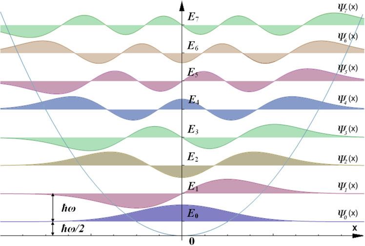
Like the one-dimensional harmonic oscillator problem, an LC circuit can be quantized by either solving the Schrödinger equation or using creation and annihilation operators. The energy stored in the inductor can be looked at as a "kinetic energy term" and the energy stored in the capacitor can be looked at as a "potential energy term".

The Hamiltonian of such a system is:

H = ϕ 2 2 L + 1 2 L ω 2 Q 2

where Q is the charge operator, and ϕ is the magnetic flux operator. The first term represents the energy stored in an inductor, and the second term represents the energy stored in a capacitor. In order to find the energy levels and the corresponding energy eigenstates, we must solve the time-independent Schrödinger equation,

H | ψ ⟩ = E | ψ ⟩   E ψ = − ℏ 2 2 L ∇ 2 ψ + 1 2 L ω 2 Q 2 ψ

Since an LC circuit really is an electrical analog to the harmonic oscillator, solving the Schrödinger equation yields a family of solutions (the Hermite polynomials).

⟨ Q | ψ n ⟩ = 1 2 n n ! ⋅ ( L ω π ℏ ) 1 / 4 ⋅ exp ⁡ ( − L ω Q 2 2 ℏ ) ⋅ H n ( L ω ℏ Q ) n = 0 , 1 , 2 , …

Magnetic Flux as a Conjugate Variable

A completely equivalent solution can be found using magnetic flux as the conjugate variable where the conjugate "momentum" is equal to capacitance times the time derivative of magnetic flux. The conjugate "momentum" is really the charge.

π = C d ϕ d t

Using Kirchhoff's Junction Rule, the following relationship can be obtained:

C d V d t + 1 L ∫ 0 t V d t = 0

Since V = d ϕ d t , the above equation can be written as follows:

C d 2 ϕ d t 2 + 1 L ϕ = 0

Converting this into a Hamiltonian, one can develop a Schrödinger equation as follows:

i ℏ d ψ d t = − ℏ 2 2 C ∇ 2 ψ + ϕ 2 2 L ψ where ψ is a function of magnetic flux

Quantization of coupled LC circuits

Two inductively coupled LC circuits have a non-zero mutual inductance. This is equivalent to a pair of harmonic oscillators with a kinetic coupling term.

The Lagrangian for an inductively coupled pair of LC circuits is as follows:

L = 1 2 L 1 d Q 1 d t 2 + 1 2 L 2 d Q 2 d t 2 + m d Q 1 d t d Q 2 d t − Q 1 2 2 C 1 − Q 2 2 2 C 2

As usual, the Hamiltonian is obtained by a Legendre transform of the Lagrangian.

H = 1 2 L 1 d Q 1 d t 2 + 1 2 L 2 d Q 2 d t 2 + m d Q 1 d t d Q 2 d t + Q 1 2 2 C 1 + Q 2 2 2 C 2

Promoting the observables to quantum mechanical operators yields the following Schrödinger equation.

E ψ = − ℏ 2 2 L 1 d 2 ψ d Q 1 2 − ℏ 2 2 L 2 d 2 ψ d Q 2 2 − ℏ 2 m d 2 ψ d Q 1 d Q 2 + 1 2 L 1 ω 2 Q 1 2 ψ + 1 2 L 2 ω 2 Q 2 2 ψ

One cannot proceed further using the above coordinates because of the coupled term. However, a coordinate transformation from the wave function as a function of both charges to the wave function as a function of the charge difference Q d , where Q d = Q 1 − Q 2 and a coordinate Q c (somewhat analogous to a "Center-of-Mass"), the above Hamiltonian can be solved using the Separation of Variables technique.

The CM coordinate is as seen below:

Q c = L 1 Q 1 + L 2 Q 2 L 1 + L 2

The Hamiltonian under the new coordinate system is as follows:

E ψ = − ℏ 2 ( 1 − λ ) 2 ( L 1 + L 2 ) d 2 ψ d Q c 2 − ℏ 2 ( 1 − λ ) 2 μ d 2 ψ d Q d 2 + 1 2 μ ω 2 Q d 2 ψ

In the above equation λ is equal to 2 m L 1 + L 2 and μ equals the reduced inductance.

The separation of variables technique yields two equations, one for the "CM" coordinate that is the differential equation of a free particle, and the other for the charge difference coordinate, which is the Schrödinger equation for a harmonic oscillator.

E ψ c = − ℏ 2 ( 1 − λ ) 2 ( L 1 + L 2 ) d 2 ψ c d Q c 2 E ψ d = − ℏ 2 ( 1 − λ ) 2 μ d 2 ψ d d Q d 2 + 1 2 μ ω 2 Q d 2 ψ d

The solution for the first differential equation once the time dependence is appended resembles a plane wave, while the solution of the second differential equation is seen above.

Classical case

Stored energy (Hamiltonian) for classical LC circuit:

H = q 2 ( t ) 2 C + p 2 ( t ) 2 L  

Hamiltonian's equations:

∂ H ( q , p ) ∂ q = q ( t ) C = − p ˙ ( t )   ∂ H ( q , p ) ∂ p = p ( t ) L = − q ˙ ( t )   ,

where q ( t ) = C v ( t )   stored capacitor charge (or electric flux) and p ( t ) = L i ( t )   magnetic momentum (magnetic flux), v ( t ) −   capacitor voltage and i ( t ) −   inductance current, t −   time variable.

Nonzero initial conditions: At q ( 0 ) , p ( 0 )   we shall have oscillation frequency:

ω = 1 L C   ,

and wave impedance of the LC circuit (without dissipation):

ρ = L C  

Hamiltonian's equations solutions: At t ≥ 0   we shall have the following values of charges, magnetic flux and energy:

q = q ( 0 ) + j p ( 0 ) ω L   < q ( t ) = R e [ q e − j ω t ]   p ( t ) = I m [ ω L q e − j ω t ]   H = | q | 2 2 C = c o n s t a n t  

Definition of the Phasor

In the general case the wave amplitudes can be defined in the complex space

a ( t ) = a 1 ( t ) + j a 2 ( t )  

where j = − 1   .

a 1 ( t ) = q ( t ) q ( 0 )   ,

where q ( 0 ) = D ( 0 ) S C = 2 ℏ ρ   - electric charge at zero time, S C −   capacitance area.

a 2 ( t ) = p ( t ) p ( 0 )   ,

where p ( 0 ) = 2 ℏ ρ   - magnetic flux at zero time, S L −   inductance area. Note that, at the equal area elements

S C = S L = S q  

we shall have the following relationship for the wave impedance:

ρ = L C = q ( 0 ) p ( 0 ) .

Wave amplitude and energy could be defined as:

a ( t ) = a e − j ω t   H = ℏ ω [ a 1 2 ( t ) + a 2 2 ( t ) ] = ℏ ω | a | 2   .

Quantum case

In the quantum case we have the following definition for momentum operator:

p ^ = − j ℏ ∂ ∂ q

Momentum and charge operators produce the following commutator:

[ q ^ , p ^ ] = j ℏ   .

Amplitude operator can be defined as:

a ^ = a 1 ^ + j a 2 ^ = q ^ q 0 + j p ^ p 0   ,

and phazor:

a ( t ) ^ = a ^ e − j ω t   .

Hamilton's operator will be:

H ^ ℏ ω [ a ^ 1 2 ( t ) + a ^ 2 2 ( t ) ] = ℏ ω [ a ^ a ^ † + 1 / 2 ]  

Amplitudes commutators:

[ a ^ 1 ( t ) , a ^ 2 ( t ) ] = j / 2   [ a ^ ( t ) , a ^ † ( t ) ] = 1   .

Heisenberg uncertainty principle:

⟨ Δ a ^ 1 2 ( t ) ⟩ ⟨ Δ a ^ 2 2 ( t ) ⟩ ≥ 1 16   .

Wave impedance of free space

When wave impedance of quantum LC circuit takes the value of free space

ρ 0 = L 0 C 0 = μ 0 ϵ 0 = 2 α h e 2 ,

where e −   electron charge and α −   fine structure constant, then "electric" and "magnetic" fluxes at zero time point will be:

q 0 = 2 ℏ ρ 0 = e 2 π α   p 0 = 2 ℏ ρ 0 = ϕ 0 2 α π   ,

where ϕ 0 = h e −   magnetic flux quantum.

General formulation

In the classical case the energy of LC circuit will be:

W L C = W C + W L ,  

where W C = 0.5 C V C 2 −   capacitance energy, and W L = 0.5 L I L 2 −   inductance energy. Furthermore, there are the following relationships between charges (electric or magnetic) and voltages or currents:

Q C = C V C   Φ L = L I L .  

Therefore, the maximal values of capacitance and inductance energies will be:

W m a x = W L C = Q C 0 2 2 C + Φ L 0 2 2 L .  

Note that the resonance frequency ω 0 = 1 / L C   has nothing to do with the energy in the classical case. But it has the following relationship with energy in the quantum case:

W 0 = ℏ ω 0 2 = ℏ 2 L C .  

So, in the quantum case, by filling capacitance with the one electron charge:

Q C 0 = e = C V C   and W C = e 2 2 C .  

The relationship between capacitance energy and the ground state oscillator energy will then be:

ξ C = W C W 0 = 2 π R H L C = 2 π ⋅ ρ q R H .  

where ρ q = L / C   quantum impedance of LC circuit. The quantum impedance of the quantum LC circuit could be in practice of the two types:

ρ q = L C = { ρ w = 2 α R H ,  - wave impedance  ρ D O S = R H ,  - DOS impedance 

So, the energy relationships will be:

ξ C = W C W 0 = 2 π ρ q R H = { 4 π α , at  ρ w 2 π , at  ρ D O S

and that is the main problem of the quantum LC circuit: energies stored on capacitance and inductance are not equal to the ground state energy of the quantum oscillator. This energy problem produces the quantum LC circuit paradox (QLCCP).

Possible solution

Some simple solution of the QLCCP could be found in the following way. Yakymakha (1989) (eqn.30) proposed the following DOS quantum impedance definition:

ρ D O S i j = Δ Φ j Δ Q i = i j R H ,  

where Δ Φ j = j Φ 0 −   magnetic flux, and Δ Q i = i e −   electric flux, i , j = i n t e g e r .

So, there are no electric or magnetic charges in the quantum LC circuit, but electric and magnetic fluxes only. Therefore, not only in the DOS LC circuit, but in the other LC circuits too, there are only the electromagnetic waves. Thus, the quantum LC circuit is the minimal geometrical-topological value of the quantum waveguide, in which there are no electric or magnetic charges, but electromagnetic waves only. Now one should consider the quantum LC circuit as a "black wave box" (BWB), which has no electric or magnetic charges, but waves. Furthermore, this BWB could be "closed" (in Bohr atom or in the vacuum for photons), or "open" (as for QHE and Josephson junction). So, the quantum LC circuit should has BWB and "input - output" supplements. The total energy balance should be calculated with considering of "input" and "output" devices. Without "input - output" devices, the energies "stored" on capacitances and inductances are virtual or "characteristics", as in the case of characteristic impedance (without dissipation). Very close to this approach now are Devoret (2004), which consider Josephson junctions with quantum inductance, Datta impedance of Schrödinger waves (2008) and Tsu (2008), which consider quantum wave guides.

Explanation for DOS quantum LC circuit

As presented below, the resonance frequency for QHE is:

ω Q = 1 L Q A C Q A = ω B 2 π ,  

where ω B = e B / m −   cyclotron frequency, L Q A = 4 π R H ω B   and C Q A = 4 π R H ω B .   The scaling current for QHE will be:

I B = e ω B 4 π .  

Therefore, the inductance energy will be:

W L = L Q A I B 2 2 = ℏ ω B 4 .  

So for quantum magnetic flux Φ 0 = h / e   , inductance energy is half as much as the ground state oscillation energy. This is due to the spin of electron (there are two electrons on Landau level on the same quantum area element). Therefore, the inductance/capacitance energy considers the total Landau level energy per spin.

Explanation for "wave" quantum LC circuit

By analogy to the DOS LC circuit, we have

W 0 = 1 2 ⋅ W C 2 π α = γ B Y W C 2  

two times lesser value due to the spin. But here there is the new dimensionless fundamental constant:

γ B Y = 1 2 π α  

which considers topological properties of the quantum LC circuit. This fundamental constant first appeared in the Bohr atom for Bohr radius:

a B = γ B Y ⋅ λ 0 ,  

where λ 0 = h / m 0 c −   Compton wavelength of electron.

Thus, the wave quantum LC circuit has no charges in it, but electromagnetic waves only. So capacitance or inductance "characteristic energies" are γ B Y −   times less than the total energy of the oscillator. In other words, charges "disappear" at the "input" and "generate" at the "output" of the wave LC circuit, adding energies to keep balance.

Total energy of quantum LC circuit

Energy stored on the quantum capacitance:

W C = Q C 2 2 C = 2 π α W L C .  

Energy stored on the quantum inductance:

W L = Φ L 2 2 L = 2 π α W L C .  

Resonance energy of the quantum LC circuit:

W L C = ℏ ω L C = ℏ L C .  

Thus, the total energy of the quantum LC circuit should be:

W t o t = W L C + W C + W L .  

In the general case, resonance energy W L C   could be due to the "rest mass" of electron, energy gap for Bohr atom, etc. However, energy stored on capacitance W C   is due to electric charge. Actually, for free electron and Bohr atom LC circuits we have quantized electric fluxes, equal to the electronic charge, e   .

Furthermore, energy stored on inductance W L   is due to magnetic momentum. Actually, for Bohr atom we have Bohr Magneton:

μ B = e ℏ 2 m 0 = 0.5 e ν B S B = e a B 2 L B C B .  

In the case of free electron, Bohr Magneton will be:

μ e = 0.5 e ν e S e = 0.5 e m 0 c 2 h λ 0 2 2 π = e ℏ 2 m 0 ,  

the same, as for Bohr atom.

Electron as LC circuit

Electron capacitance could be presented as the spherical capacitor:

C e = 4 π ϵ 0 1 r e − 1 r e + λ 0 = ϵ 0 λ 0 2 π ,  

where r e = λ 0 2 2 π −   electron radius and λ 0 −   Compton wavelength.

Note, that this electron radius is consistent with the standard definition of the spin. Actually, rotating momentum of electron is:

l e = m 0 ω e r e 2 = ℏ / 2 ,  

where ω e = m 0 c 2 / ℏ   is considered.

Spherical inductance of electron:

L e = μ 0 λ 0 2 π .  

Characterictic impedance of electron:

ρ e = L e C e = μ 0 ϵ 0 = ρ 0 = 2 α R H .  

Resonance frequency of electron LC circuit:

ω e = 1 L e C e = 2 π c λ 0 = m 0 c 2 ℏ .  

Induced electric flux on electron capacitance:

Q e = C e V e .  

Energy, stored on electron capacitance:

W C e = C e V e 2 2 = Q e 2 2 C e = 2 π α W 0 ,  

where W 0 = m 0 c 2 −   is the "rest energy" of electron. So, induced electric flux will be:

Q e = 2 α m 0 c 2 ϵ 0 λ 0 = e .  

Thus, through electron capacitance we have quantized electric flux, equal to the electron charge.

Magnetic flux through inductance:

Φ e = L e I e .  

Magnetic energy, stored on inductance:

W L e = L e I e 2 2 = Φ e 2 2 L e = 2 π α W 0 .  

So, induced magnetic flux will be:

Φ e = 2 μ 0 h c α = 2 α Φ 0 .  

where Φ 0 = h / e −   magnetic flux quantum. Thus, through electron inductance there are no quantization of magnetic flux.

Bohr atom as LC circuit

Bohr radius:

a B = λ 0 2 π α  

where λ 0 = h m 0 c −   Compton wavelength of electron, α −   fine structure constant.

Bohr atomic surface:

S B = 4 π a B 2   .

Bohr inductance:

L B = μ 0 λ 0 ⋅ S B   .

Bohr capacitance:

C B = ϵ 0 λ 0 ⋅ S B   .

Bohr wave impedance:

ρ B = L B C B = μ 0 ϵ 0 = ρ 0 .  

Bohr angular frequency:

ω B = 1 L B C B = α 2 2 ⋅ m 0 c 2 ℏ = 2 π c λ B ,  

where λ B = 4 π a B α −   Bohr wavelength for the first energy level.

Induced electric flux of the Bohr first energy level:

Q B = C B V B .  

Energy, stored on the Bohr capacitance:

W C B = C B V B 2 2 = Q B 2 2 C B = 2 π α W B ,  

where W B = ℏ ω B −   is the Bohr energy. So, induced electric flux will be:

Q B = 2 π α 3 m 0 c 2 C B = e .  

Thus, through the Bohr capacitance we have quantized electric flux, equal to the electron charge.

Magnetic flux through the Bohr inductance:

W L B = L B I B 2 2 = Φ B 2 2 L B = 2 π α W 0 .  

So, induced magnetic flux will be:

Φ B = π α 2 e c λ 0 L B = 2 α Φ 0 .  

Thus, through the Bohr inductance there are no quantization of magnetic flux.

Photon as LC circuit

Photon "resonant angular frequency":

ω w = 1 L w C w .  

Photon "wave impedance":

ρ w = L w C w = μ 0 ϵ 0 = ρ 0 .  

Photon "wave inductance":

L w = ρ 0 ω w .  

Photon "wave capacitance":

C w = 1 ρ 0 ω w .  

Photon "magnetic flux quantum":

ϕ w = L w I w = ϕ 0 = h e .  

Photon "wave current":

I w = h e L w = e ω w 2 α .  

Quantum Hall effect as LC circuit

In the general case 2D- density of states (DOS) in a solid could be defined by the following:

D 2 D = m ∗ π ℏ 2   ,

where m ∗ = ξ m 0 −   current carriers effective mass in a solid, m 0 −   electron mass, and ξ −   dimensionless parameter, which considers band structure of a solid. So, the quantum inductance can be defined as follows:

L Q L = ϕ 0 2 ⋅ D 2 D = ξ ⋅ L Q 0 ,

where L Q 0 8 π β ⋅ L Q Y   - the ‘’ideal value’’ of quantum inductance at ξ = 1   and another ideal quantum inductance:

L Q Y = μ 0 λ 0 = H / m 2   , (3)

where μ 0 −   magnetic constant, β = 1 4 α −   magnetic "fine structure constant"(p. 62), α −   fine structure constant and λ 0 −   Compton wavelength of electron, first defined by Yakymakha (1994) in the spectroscopic investigations of the silicon MOSFETs.

Since defined above quantum inductance is per unit area, therefore its absolute value will be in the QHE mode:

L Q A = L Q L n B   ,

where the carrier concentration is:

n B = e B h   ,

and h −   is the Planck constant. By analogically, the absolute value of the quantum capacitance will be in the QHE mode:

C Q A = C Q L n B   ,

where

C Q L = e 2 ⋅ D 2 D = ξ ⋅ C Q 0 ,

is DOS definition of the quantum capacitance according to Luryi, C Q 0 = 8 π α ⋅ C Q Y   - quantum capacitance ‘’ideal value’’ at ξ = 1   , and other quantum capacitance:

C Q Y = ϵ 0 λ 0 = 3.6492417 F / m 2   ,

where ϵ 0 −   dielectric constant, first defined by Yakymakha (1994) > in the spectroscopic investigations of the silicon MOSFETs. The standard wave impedance definition for the QHE LC circuit could be presented as:

ρ Q = L Q A C Q A = ϕ 0 2 e 2 = h e 2 = R H   ,

where R H = h e 2 = 25.812813 k Ω   von Klitzing constant for resistance.

The standard resonant frequency definition for the QHE LC circuit could be presented as:

ω Q = 1 L Q A C Q A = ℏ ω c ϕ 0 e = ω c 2 π ,

where ω c = e B m ∗ −   standard cyclotron frequency in the magnetic field B.

Hall scaling current quantum will be

I H = h e L Q A = e ω B 4 π   ,

where ω B = e B m ∗ −   Hall angular frequency.

Josephson junction as LC circuit

Electromagnetic induction (Faraday) low:

V i n d = ∂ Φ ∂ t = − L ∂ I ∂ t ,  

where Φ −   magnetic flux, L −   Josephson junction quantum inductance and I −   Josephson junction current. DC Josephson equation for current:

I = I J ⋅ sin ⁡ ϕ ,  

where I J −   Josephson scale for current, ϕ −   phase difference between superconductors. Current derivative on time variable will be:

∂ I ∂ t = I J cos ⁡ ϕ ⋅ ∂ ϕ ∂ t .  

AC Josephson equation:

∂ ϕ ∂ t = q ℏ V = 2 π Φ 0 V ,  

where ℏ −   reduced Planck constant, Φ 0 = h / 2 e − Josephson magnetic flux quantum, q = 2 e   and e −   electron charge. Combining equations for derivatives yields junction voltage:

V = Φ 0 2 π I J ⋅ 1 cos ⁡ ϕ ⋅ ∂ I ∂ t = L J ⋅ ∂ I ∂ t ,  

where

L J = Φ 0 2 π I J ⋅ 1 cos ⁡ ϕ  

is the Devoret (1997) quantum inductance.

AC Josephson equation for angular frequency:

ω J = q ℏ ⋅ V .  

Resonance frequency for Josephson LC circuit:

ω J = 1 L J C J .  

where C J −   is the Devoret quantum capacitance, that can be defined as:

C J = 1 L J ω J 2 = Φ 0 I J V 0 2 ⋅ cos ⁡ ϕ 2 π .  

Quantum wave impedance of Josephson junction:

ρ J = L J C J = V 0 I J ⋅ 1 cos ⁡ ϕ .  

For V 0 = 0 , 1 mV and I J = 0 , 2 μ A wave impedance will be ρ J = 500 Ω .  

Flat Atom as LC circuit

Quantum capacitance of Flat Atom (FA):

C F 0 = ϵ 0 λ 0 ⋅ S F 0 = 5.1805 ⋅ 10 − 7   F,

where λ 0 = h m 0 c   .

Quantum inductance of FA:

L F 0 = μ 0 λ 0 ⋅ S F 0 = 7.3524 ⋅ 10 − 2   H.

Quantum area element of FA:

S F 0 = λ 0 c ω F 0 = h m 0 ω F 0 = 1.4196 ⋅ 10 − 7   m².

Resonance frequency of FA:

ω F 0 = 1 L F 0 C F 0 = 5123.9   rad/s.

Characteristic impedunce of FA:

ρ F 0 = L F 0 C F 0 = ρ 0 = 2 α R H ,  

where ρ 0   is the impedance of free space.

Total electric charge on the first energy level of FA:

Q F 1 = e S F 0 S B = 2 ⋅ 10 6 e   ,

where S B = 4 π a B 2 −   Bohr quantum area element. First FA was discovered by Yakymakha (1994) as very low frequency resonance on the p- channel MOSFETs. Contrary to the spherical Bohr atom, the FA has gyperbolic dependence on the number of energy level (n)

ω F 0 n = ω F 0 n .