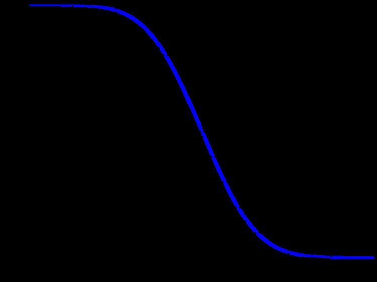
In statistics, the Q-function is the tail probability of the standard normal distribution ϕ ( x ) . In other words, Q(x) is the probability that a normal (Gaussian) random variable will obtain a value larger than x standard deviations above the mean.
If the underlying random variable is y, then the proper argument to the tail probability is derived as:
x = y − μ σ which expresses the number of standard deviations away from the mean.
Other definitions of the Q-function, all of which are simple transformations of the normal cumulative distribution function, are also used occasionally.
Because of its relation to the cumulative distribution function of the normal distribution, the Q-function can also be expressed in terms of the error function, which is an important function in applied mathematics and physics.
Definition and basic properties
Formally, the Q-function is defined as
Q ( x ) = 1 2 π ∫ x ∞ exp ( − u 2 2 ) d u . Thus,
Q ( x ) = 1 − Q ( − x ) = 1 − Φ ( x ) , where Φ ( x ) is the cumulative distribution function of the normal Gaussian distribution.
The Q-function can be expressed in terms of the error function, or the complementary error function, as
Q ( x ) = 1 2 ( 2 π ∫ x / 2 ∞ exp ( − t 2 ) d t ) = 1 2 − 1 2 erf ( x 2 ) -or- = 1 2 erfc ( x 2 ) . An alternative form of the Q-function known as Craig's formula, after its discoverer, is expressed as:
Q ( x ) = 1 π ∫ 0 π 2 exp ( − x 2 2 sin 2 θ ) d θ . This expression is valid only for positive values of x, but it can be used in conjunction with Q(x) = 1 − Q(−x) to obtain Q(x) for negative values. This form is advantageous in that the range of integration is fixed and finite.
The Q-function is not an elementary function. However, the boundsbecome increasingly tight for large
x, and are often useful.Using the
substitution v =
u2/2, the upper bound is derived as follows:Similarly, using
ϕ ′ ( u ) = − u ϕ ( u ) and the
quotient rule,Solving for
Q(
x) provides the lower bound.
The Chernoff bound of the Q-function isImproved exponential bounds and a pure exponential approximation are A tight approximation of Q ( x ) for x ∈ [ 0 , ∞ ) is given by Karagiannidis & Lioumpas (2007) who showed for the appropriate choice of parameters { A , B } that f ( x ; A , B ) = ( 1 − e − A x ) e − x 2 B π x ≈ erfc ( x ) . The absolute error between
f ( x ; A , B ) and
erfc ( x ) over the range
[ 0 , R ] is minimized by evaluating
{ A , B } = a r g m i n { A , B } 1 R ∫ 0 R | f ( x ; A , B ) − erfc ( x ) | d x . Using
R = 20 and numerically integrating, they found the minimum error occurred when
{ A , B } = { 1.98 , 1.135 } , which gave a good approximation for
∀ x ≥ 0. Substituting these values and using the relationship between
Q ( x ) and
erfc ( x ) from above gives
Q ( x ) ≈ ( 1 − e − 1.4 x ) e − x 2 2 1.135 2 π x , x ≥ 0. Inverse Q
The inverse Q-function can be related to the inverse error functions:
Q − 1 ( y ) = 2 e r f − 1 ( 1 − 2 y ) = 2 e r f c − 1 ( 2 y ) The function Q − 1 ( y ) finds application in digital communications. It is usually expressed in dB and generally called Q-factor:
Q - f a c t o r = 20 log 10 ( Q − 1 ( y ) ) d B where y is the bit-error rate (BER) of the digitally modulated signal under analysis. For instance, for QPSK in additive white Gaussian noise, the Q-factor defined above coincides with the value in dB of the signal to noise ratio that yields a bit error rate equal to y.
The Q-function is well tabulated and can be computed directly in most of the mathematical software packages such as R and those available in Python, MATLAB and Mathematica. Some values of the Q-function are given below for reference.
The Q-function can be generalized to higher dimensions:
Q ( x ) = P ( X ≥ x ) , where X ∼ N ( 0 , Σ ) follows the multivariate normal distribution with covariance Σ and the threshold is of the form x = γ Σ l ∗ for some positive vector l ∗ > 0 and positive constant γ > 0 . As in the one dimensional case, there is no simple analytical formula for the Q-function. Nevertheless, the Q-function can be approximated arbitrarily well as γ becomes larger and larger.