
 | ||
Support x ∈ [ 0 ; + ∞ ) for q ≥ 1 {displaystyle xin [0;+infty )!{ ext{ for }}qgeq 1} x ∈ [ 0 ; 1 λ ( 1 − q ) ) for q < 1 {displaystyle xin [0;{1 over {lambda (1-q)}}){ ext{ for }}q<1} PDF ( 2 − q ) λ e q − λ x {displaystyle {(2-q)lambda e_{q}^{-lambda x}}} CDF 1 − e q ′ − λ x q ′ where q ′ = 1 2 − q {displaystyle {1-e_{q'}^{-lambda x over q'}}{ ext{ where }}q'={1 over {2-q}}} Mean 1 λ ( 3 − 2 q ) for q < 3 2 {displaystyle {1 over lambda (3-2q)}{ ext{ for }}q<{3 over 2}} Otherwise undefined Median − q ′ ln q ′ ( 1 2 ) λ where q ′ = 1 2 − q {displaystyle {{-q'{ ext{ ln}}_{q'}({1 over 2})} over {lambda }}{ ext{ where }}q'={1 over {2-q}}} | ||
The q-exponential distribution is a probability distribution arising from the maximization of the Tsallis entropy under appropriate constraints, including constraining the domain to be positive. It is one example of a Tsallis distribution. The q-exponential is a generalization of the exponential distribution in the same way that Tsallis entropy is a generalization of standard Boltzmann–Gibbs entropy or Shannon entropy. The exponential distribution is recovered as
Contents
- Probability density function
- Derivation
- Relationship to other distributions
- Generating random deviates
- Applications
- References
Originally proposed by the statisticians George Box and David Cox in 1964, and known as the reverse Box–Cox transformation for
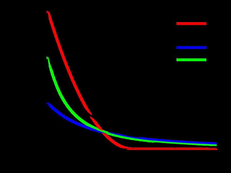
Probability density function
The q-exponential distribution has the probability density function
where
is the q-exponential, if q≠1. When q=1, eq(x) is just exp(x).
Derivation
In a similar procedure to how the exponential distribution can be derived using the standard Boltzmann–Gibbs entropy or Shannon entropy and constraining the domain of the variable to be positive, the q-exponential distribution can be derived from a maximization of the Tsallis Entropy subject to the appropriate constraints.
Relationship to other distributions
The q-exponential is a special case of the generalized Pareto distribution where
The q-exponential is the generalization of the Lomax distribution (Pareto Type II), as it extends this distribution to the cases of finite support. The Lomax parameters are:
As the Lomax distribution is a shifted version of the Pareto distribution, the q-exponential is a shifted reparameterized generalization of the Pareto. When q > 1, the q-exponential is equivalent to the Pareto shifted to have support starting at zero. Specifically:
Generating random deviates
Random deviates can be drawn using inverse transform sampling. Given a variable U that is uniformly distributed on the interval (0,1), then
where
Applications
Being a power transform, it is a usual technique in statistics for stabilizing the variance, making the data more normal distribution-like and improving the validity of measures of association such as the Pearson correlation between variables.