Generalized Pareto distribution - Alchetron, the free social encyclopedia



Parameters μ ∈ ( − ∞ , ∞ ) {\displaystyle \mu \in (-\infty ,\infty )\,} location (real) σ ∈ ( 0 , ∞ ) {\displaystyle \sigma \in (0,\infty )\,} scale (real) ξ ∈ ( − ∞ , ∞ ) {\displaystyle \xi \in (-\infty ,\infty )\,} shape (real) Support x ⩾ μ ( ξ ⩾ 0 ) {\displaystyle x\geqslant \mu \,\;(\xi \geqslant 0)} μ ⩽ x ⩽ μ − σ / ξ ( ξ < 0 ) {\displaystyle \mu \leqslant x\leqslant \mu -\sigma /\xi \,\;(\xi <0)} PDF 1 σ ( 1 + ξ z ) − ( 1 / ξ + 1 ) {\displaystyle {\frac {1}{\sigma }}(1+\xi z)^{-(1/\xi +1)}} where z = x − μ σ {\displaystyle z={\frac {x-\mu }{\sigma }}} CDF 1 − ( 1 + ξ z ) − 1 / ξ {\displaystyle 1-(1+\xi z)^{-1/\xi }\,} Mean μ + σ 1 − ξ ( ξ < 1 ) {\displaystyle \mu +{\frac {\sigma }{1-\xi }}\,\;(\xi <1)} Median μ + σ ( 2 ξ − 1 ) ξ {\displaystyle \mu +{\frac {\sigma (2^{\xi }-1)}{\xi }}}

In statistics, the generalized Pareto distribution (GPD) is a family of continuous probability distributions. It is often used to model the tails of another distribution. It is specified by three parameters: location μ , scale σ , and shape ξ . Sometimes it is specified by only scale and shape and sometimes only by its shape parameter. Some references give the shape parameter as κ = − ξ .

Definition

The standard cumulative distribution function (cdf) of the GPD is defined by

F ξ ( z ) = { 1 − ( 1 + ξ z ) − 1 / ξ for ξ ≠ 0 , 1 − e − z for ξ = 0.

where the support is z ≥ 0 for ξ ≥ 0 and 0 ≤ z ≤ − 1 / ξ for ξ < 0 .

f ξ ( z ) = { ( ξ z + 1 ) − ξ + 1 ξ for ξ ≠ 0 , e − z for ξ = 0.

Differential equation

The cdf of the GPD is a solution of the following differential equation:

{ ( ξ z + 1 ) f ξ ′ ( z ) + ( ξ + 1 ) f ξ ( z ) = 0 , f ξ ( 0 ) = 1 }

Characterization

The related location-scale family of distributions is obtained by replacing the argument z by x − μ σ and adjusting the support accordingly: The cumulative distribution function is

F ( ξ , μ , σ ) ( x ) = { 1 − ( 1 + ξ ( x − μ ) σ ) − 1 / ξ for ξ ≠ 0 , 1 − exp ⁡ ( − x − μ σ ) for ξ = 0.

for x ⩾ μ when ξ ⩾ 0 , and μ ⩽ x ⩽ μ − σ / ξ when ξ < 0 , where μ ∈ R , σ > 0 , and ξ ∈ R .

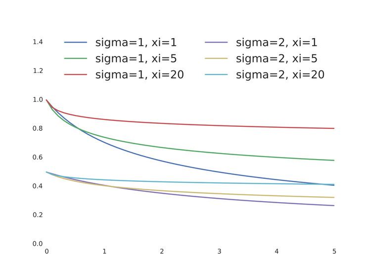
The probability density function (pdf) is

f ( ξ , μ , σ ) ( x ) = 1 σ ( 1 + ξ ( x − μ ) σ ) ( − 1 ξ − 1 ) ,

or equivalently

f ( ξ , μ , σ ) ( x ) = σ 1 ξ ( σ + ξ ( x − μ ) ) 1 ξ + 1 ,

again, for x ⩾ μ when ξ ⩾ 0 , and μ ⩽ x ⩽ μ − σ / ξ when ξ < 0 .

The pdf is a solution of the following differential equation:

{ f ′ ( x ) ( − μ ξ + σ + ξ x ) + ( ξ + 1 ) f ( x ) = 0 , f ( 0 ) = ( 1 − μ ξ σ ) − 1 ξ − 1 σ }

Characteristic and Moment Generating Functions

The characteristic and moment generating functions are derived and skewness and kurtosis are obtained from MGF by Muraleedharan and Guedes Soares

Special cases

If the shape ξ and location μ are both zero, the GPD is equivalent to the exponential distribution.

With shape ξ > 0 and location μ = σ / ξ , the GPD is equivalent to the Pareto distribution with scale x m = σ / ξ and shape α = 1 / ξ .

GPD is quite similar to the Burr distribution.

Generating generalized Pareto random variables

If U is uniformly distributed on (0, 1], then

X = μ + σ ( U − ξ − 1 ) ξ ∼ GPD ( μ , σ , ξ ≠ 0 )

and

X = μ − σ ln ⁡ ( U ) ∼ GPD ( μ , σ , ξ = 0 ) .

Both formulas are obtained by inversion of the cdf.

In Matlab Statistics Toolbox, you can easily use "gprnd" command to generate generalized Pareto random numbers.

References

Generalized Pareto distribution Wikipedia

(Text) CC BY-SA

Contents