Pulsed electron paramagnetic resonance

Scope

Electron paramagnetic resonance (EPR) or electron spin resonance (ESR) is a spectroscopic technique widely used in biology, chemistry, medicine and physics to study systems with one or more unpaired electrons. Because of the specific relation between the magnetic parameters, electronic wavefunction and the configuration of the surrounding non-zero spin nuclei, EPR and ENDOR provide information on the structure, dynamics and the spatial distribution of the paramagnetic species. However, these techniques are limited in spectral and time resolution when used with traditional continuous wave methods. This resolution can be improved in pulsed EPR by investigating interactions separately from each other via pulse sequences.

Historical overview

R. J. Blume reported the first electron spin echo in 1958, which came from a solution of sodium in ammonia at room temperature. A magnetic field of 0.62 mT was used requiring a frequency of 17.4 MHz. The first microwave electron spin echoes were reported in the same year by Gordon and Bowers using 23 GHz excitation of dopants in silicon.

Much of the pioneering early pulsed EPR was conducted in the group of W. B. Mims at Bell Labs during the 1960s. In the first decade only a small number of groups worked the field, because of the expensive instrumentation, the lack of suitable microwave components and slow digital electronics. The first observation of electron spin echo envelope modulation (ESEEM) was made in 1961 by Mims, Nassau and McGee. Pulsed electron nuclear double resonance (ENDOR) was invented in 1965 by Mims. In this experiment, pulsed NMR transitions are detected with pulsed EPR. ESEEM and pulsed ENDOR continue to be important for studying nuclear spins coupled to electron spins.

In the 1980s, the upcoming of the first commercial pulsed EPR and ENDOR spectrometers in the X band frequency range, lead to a fast growth of the field. In the 1990s, parallel to the upcoming high-field EPR, pulsed EPR and ENDOR became a new fast advancing magnetic resonance spectroscopy tool and the first commercial pulsed EPR and ENDOR spectrometer at W band frequencies appeared on the market.

Principle

The basic principle of pulsed EPR is similar to NMR spectroscopy. Differences can be found in the relative size of the magnetic interactions and in the relaxation rates which are orders of magnitudes larger in EPR than NMR. A full description of the theory is given within the quantum mechanical formalism, but since the magnetization is being measured as a bulk property, a more intuitive picture can be obtained with a classical description. For a better understanding of the concept of pulsed EPR let us consider the effects on the magnetization vector in the laboratory frame as well as in the rotating frame. As the animation below shows, in the laboratory frame the static magnetic field B₀ is assumed to be parallel to the z-axis and the microwave field B₁ parallel to the x-axis. When an electron spin is placed in magnetic field it experiences a torque which causes its magnetic moment to precess around the magnetic field. The precession frequency is known as the Larmor frequency ω_L (see page 18 of ref ).

where γ is the gyromagnetic ratio and B₀ the magnetic field. The electron spins are characterized by two quantum mechanical states, one parallel and one antiparallel to B₀. Because of the lower energy of the parallel state more electron spins can be found in this state according to the Boltzmann distribution. This results in a net magnetization, which is the vector sum of all magnetic moments in the sample, parallel to the z-axis and the magnetic field. To better comprehend the effects of the microwave field B₁ it is easier to move to the rotating frame.

EPR experiments usually use a microwave resonator designed to create a linearly polarized microwave field B₁, perpendicular to the much stronger applied magnetic field B₀. The rotating frame is fixed to the rotating B₁ components. First we assume to be on resonance with the precessing magnetization vector M₀.

Therefore, the component of B₁ will appear stationary. In this frame also the precessing magnetization components appear to be stationary that leads to the disappearance of B₀, and we need only to consider B₁ and M₀. The M₀ vector is under the influence of the stationary field B₁, leading to another precession of M₀, this time around B₁ at the frequency ω₁.

This angular frequency ω₁ is also called the Rabi frequency. Assuming B₁ to be parallel to the x-axis, the magnetization vector will rotate around the +x-axis in the zy-plane as long as the microwaves are applied. The angle by which M₀ is rotated is called the tip angle α and is given by:

Here t_p is the duration for which B₁ is applied, also called the pulse length. The pulses are labeled by the rotation of M₀ which they cause and the direction from which they are coming from, since the microwaves can be phase-shifted from the x-axis on to the y-axis. For example, a +y π/2 pulse means that a B₁ field, which has been 90 degrees phase-shifted out of the +x into the +y direction, has rotated M₀ by a tip angle of π/2, hence the magnetization would end up along the –x-axis. That means the end position of the magnetization vector M₀ depends on the length, the magnitude and direction of the microwave pulse B₁. In order to understand how the sample emits microwaves after the intense microwave pulse we need to go back to the laboratory frame. In the rotating frame and on resonance the magnetization appeared to be stationary along the x or y-axis after the pulse. In the laboratory frame it becomes a rotating magnetization in the x-y plane at the Larmor frequency. This rotation generates a signal which is maximized if the magnetization vector is exactly in the xy-plane. This microwave signal generated by the rotating magnetization vector is called free induction decay (FID) (see page 175 of ref ).

Another assumption we have made was the exact resonance condition, in which the Larmor frequency is equal to the microwave frequency. In reality EPR spectra have many different frequencies and not all of them can be exactly on resonance, therefore we need to take off-resonance effects into account. The off-resonance effects lead to three main consequences. The first consequence can be better understood in the rotating frame. A π/2 pulse leaves magnetization in the xy-plane, but since the microwave field (and therefore the rotating frame) do not have the same frequency as the precessing magnetization vector, the magnetization vector rotates in the xy-plane, either faster or slower than the microwave magnetic field B₁. The rotation rate is governed by the frequency difference Δω.

If Δω is 0 then the microwave field rotates as fast as the magnetization vector and both appear to be stationary to each other. If Δω>0 then the magnetization rotates faster than the microwave field component in a counter-clockwise motion and if Δω<0 then the magnetization is slower and rotates clockwise. This means that the individual frequency components of the EPR spectrum, will appear as magnetization components rotating in the xy-plane with the rotation frequency Δω. The second consequence appears in the laboratory frame. Here B₁ tips the magnetization differently out of the z-axis, since B₀ does not disappear when not on resonance due to the precession of the magnetization vector at Δω. That means that the magnetization is now tipped by an effective magnetic field B_eff, which originates from the vector sum of B₁ and B₀. The magnetization is then tipped around B_eff at a faster effective rate ω_eff.

This leads directly to the third consequence that the magnetization can not be efficiently tipped into the xy-plane because B_eff does not lie in the xy-plane, as B₁ does. The motion of the magnetization now defines a cone. That means as Δω becomes larger, the magnetization is tipped less effectively into the xy-plane, and the FID signal decreases. In broad EPR spectra where Δω > ω₁ it is not possible to tip all the magnetization into the xy-plane to generate a strong FID signal. This is why it is important to maximize ω₁ or minimize the π/2 pulse length for broad EPR signals.

So far the magnetization was tipped into the xy-plane and it remained there with the same magnitude. However, in reality the electron spins interact with their surroundings and the magnetization in the xy-plane will decay and eventually return to alignment with the z-axis. This relaxation process is described by the spin-lattice relaxation time T₁, which is a characteristic time needed by the magnetization to return to the z-axis, and by the spin-spin relaxation time T₂, which describes the vanishing time of the magnetization in the xy-plane. The spin-lattice relaxation results from the urge of the system to return to thermal equilibrium after it has been perturbed by the B₁ pulse. Return of the magnetization parallel to B₀ is achieved through interactions with the surroundings, that is spin-lattice relaxation. The corresponding relaxation time needs to be considered when extracting a signal from noise, where the experiment needs to be repeated several times, as quickly as possible. In order to repeat the experiment, one needs to wait until the magnetization along the z-axis has recovered, because if there is no magnetization in z direction, then there is nothing to tip into the xy-plane to create a significant signal.

The spin-spin relaxation time, also called the transverse relaxation time, is related to homogeneous and inhomogeneous broadening. An inhomogeneous broadening results from the fact that the different spins experience local magnetic field inhomogeneities (different surroundings) creating a large number of spin packets characterized by a distribution of Δω. As the net magnetization vector precesses, some spin packets slow down due to lower fields and others speed up due to higher fields leading to a fanning out of the magnetization vector that results in the decay of the EPR signal. The other packets contribute to the transverse magnetization decay due to the homogeneous broadening. In this process all the spin in one spin packet experience the same magnetic field and interact with each other that can lead to mutual and random spin flip-flops. These fluctuations contribute to a faster fanning out of the magnetization vector.

All the information about the frequency spectrum is encoded in the motion of the transverse magnetization. The frequency spectrum is reconstructed using the time behavior of the transverse magnetization made up of y- and x-axis components. It is convenient that these two can be treated as the real and imaginary components of a complex quantity and use the Fourier theory to transform the measured time domain signal into the frequency domain representation. This is possible because both the absorption (real) and the dispersion (imaginary) signals are detected.

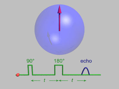
The FID signal decays away and for very broad EPR spectra this decay is rather fast due to the inhomogeneous broadening. To obtain more information one can recover the disappeared signal with another microwave pulse to produce a Hahn echo. After applying a π/2 pulse (90°), the magnetization vector is tipped into the xy-plane producing an FID signal. Different frequencies in the EPR spectrum (inhomogeneous broadening) cause this signal to "fan out", meaning that the slower spin-packets trail behind the faster ones. After a certain time t, a π pulse (180°) is applied to the system inverting the magnetization, and the fast spin-packets are then behind catching up with the slow spin-packets. A complete refocusing of the signal occurs then at time 2t. An accurate echo caused by a second microwave pulse can remove all inhomogeneous broadening effects. After all of the spin-packets bunch up, they will dephase again just like an FID. In other words, a spin echo is a reversed FID followed by a normal FID, which can be Fourier transformed to obtain the EPR spectrum. The longer the time between the pulses becomes, the smaller the echo will be due to spin relaxation. When this relaxation leads to an exponential decay in the echo height, the decay constant is the phase memory time T_M, which can have many contributions such as transverse relaxation, spectral, spin and instantaneous diffusion. Changing the times between the pulses leads to a direct measurement of T_M as shown in the spin echo decay animation below.

Applications

ESEEM and pulsed ENDOR are widely used echo experiments, in which the interaction of electron spins with the nuclei in their environment can be studied and controlled. Quantum computing and spintronics, in which spins are used to store information, have led to new lines of research in pulsed EPR.

One of the most popular pulsed EPR experiments currently is double electron-electron resonance (DEER), which is also known as pulsed electron-electron double resonance (PELDOR). This uses two different frequencies to control different spins in order to find out the strength of their coupling. The distance between the spins can then be inferred from their coupling strength, which is used to study structures of large bio-molecules.