Preconditioner

Preconditioning for linear systems

In linear algebra and numerical analysis, a preconditioner P of a matrix A is a matrix such that P − 1 A has a smaller condition number than A . It is also common to call T = P − 1 the preconditioner, rather than P , since P itself is rarely explicitly available. In modern preconditioning, the application of T = P − 1 , i.e., multiplication of a column vector, or a block of column vectors, by T = P − 1 , is commonly performed by rather sophisticated computer software packages in a matrix-free fashion, i.e., where neither P , nor T = P − 1 (and often not even A ) are explicitly available in a matrix form.

Preconditioners are useful in iterative methods to solve a linear system A x = b for x since the rate of convergence for most iterative linear solvers increases as the condition number of a matrix decreases as a result of preconditioning. Preconditioned iterative solvers typically outperform direct solvers, e.g., Gaussian elimination, for large, especially for sparse, matrices. Iterative solvers can be used as matrix-free methods, i.e. become the only choice if the coefficient matrix A is not stored explicitly, but is accessed by evaluating matrix-vector products.

Description

Instead of solving the original linear system above, one may solve either the right preconditioned system:

via solving

for y and

for x .

Alternatively, one may solve the left preconditioned system:

Both of systems give the same solution as the original system so long as the preconditioner matrix P is nonsingular. The left preconditioning is more common.

The goal of this preconditioned system is to reduce the condition number of the left or right preconditioned system matrix P − 1 A or A P − 1 , respectively. The preconditioned matrix P − 1 A or A P − 1 is almost never explicitly formed. Only the action of applying the preconditioner solve operation P − 1 to a given vector need to be computed in iterative methods.

Typically there is a trade-off in the choice of P . Since the operator P − 1 must be applied at each step of the iterative linear solver, it should have a small cost (computing time) of applying the P − 1 operation. The cheapest preconditioner would therefore be P = I since then P − 1 = I . Clearly, this results in the original linear system and the preconditioner does nothing. At the other extreme, the choice P = A gives P − 1 A = A P − 1 = I , which has optimal condition number of 1, requiring a single iteration for convergence; however in this case P − 1 = A − 1 , and applying the preconditioner is as difficult as solving the original system. One therefore chooses P as somewhere between these two extremes, in an attempt to achieve a minimal number of linear iterations while keeping the operator P − 1 as simple as possible. Some examples of typical preconditioning approaches are detailed below.

Preconditioned iterative methods

Preconditioned iterative methods for A x − b = 0 are, in most cases, mathematically equivalent to standard iterative methods applied to the preconditioned system P − 1 ( A x − b ) = 0. For example, the standard Richardson iteration for solving A x − b = 0 is

Applied to the preconditioned system P − 1 ( A x − b ) = 0 , it turns into a preconditioned method

Examples of popular preconditioned iterative methods for linear systems include the preconditioned conjugate gradient method, the biconjugate gradient method, and generalized minimal residual method. Iterative methods, which use scalar products to compute the iterative parameters, require corresponding changes in the scalar product together with substituting P − 1 ( A x − b ) = 0 for A x − b = 0.

Geometric interpretation

For a symmetric positive definite matrix A the preconditioner P is typically chosen to be symmetric positive definite as well. The preconditioned operator P − 1 A is then also symmetric positive definite, but with respect to the P -based scalar product. In this case, the desired effect in applying a preconditioner is to make the quadratic form of the preconditioned operator P − 1 A with respect to the P -based scalar product to be nearly spherical [1].

Variable and non-linear preconditioning

Denoting T = P − 1 , we highlight that preconditioning is practically implemented as multiplying some vector r by T , i.e., computing the product T r . In many applications, T is not given as a matrix, but rather as an operator T ( r ) acting on the vector r . Some popular preconditioners, however, change with r and the dependence on r may not be linear. Typical examples involve using non-linear iterative methods, e.g., the conjugate gradient method, as a part of the preconditioner construction. Such preconditioners may be practically very efficient, however, their behavior is hard to predict theoretically.

Spectrally equivalent preconditioning

The most common use of preconditioning is for iterative solution of linear systems resulting from approximations of partial differential equations. The better the approximation quality, the larger the matrix size is. In such a case, the goal of optimal preconditioning is, on the one side, to make the spectral condition number of P − 1 A to be bounded from above by a constant independent of the matrix size, which is called spectrally equivalent preconditioning by D'yakonov. On the other hand, the cost of application of the P − 1 should ideally be proportional (also independent of the matrix size) to the cost of multiplication of A by a vector.

Jacobi (or diagonal) preconditioner

The Jacobi preconditioner is one of the simplest forms of preconditioning, in which the preconditioner is chosen to be the diagonal of the matrix P = d i a g ( A ) . Assuming A i i ≠ 0 , ∀ i , we get P i j − 1 = δ i j A i j . It is efficient for diagonally dominant matrices A .

SPAI

The Sparse Approximate Inverse preconditioner minimises ∥ A T − I ∥ F , where ∥ ⋅ ∥ F is the Frobenius norm and T = P − 1 is from some suitably constrained set of sparse matrices. Under the Frobenius norm, this reduces to solving numerous independent least-squares problems (one for every column). The entries in T must be restricted to some sparsity pattern or the problem remains as difficult and time-consuming as finding the exact inverse of A . The method was introduced by M.J. Grote and T. Huckle together with an approach to selecting sparsity patterns.

Other preconditioners

External links

Preconditioning for eigenvalue problems

Eigenvalue problems can be framed in several alternative ways, each leading to its own preconditioning. The traditional preconditioning is based on the so-called spectral transformations. Knowing (approximately) the targeted eigenvalue, one can compute the corresponding eigenvector by solving the related homogeneous linear system, thus allowing to use preconditioning for linear system. Finally, formulating the eigenvalue problem as optimization of the Rayleigh quotient brings preconditioned optimization techniques to the scene.

Spectral transformations

By analogy with linear systems, for an eigenvalue problem A x = λ x one may be tempted to replace the matrix A with the matrix P − 1 A using a preconditioner P . However, this makes sense only if the seeking eigenvectors of A and P − 1 A are the same. This is the case for spectral transformations.

The most popular spectral transformation is the so-called shift-and-invert transformation, where for a given scalar α , called the shift, the original eigenvalue problem A x = λ x is replaced with the shift-and-invert problem ( A − α I ) − 1 x = μ x . The eigenvectors are preserved, and one can solve the shift-and-invert problem by an iterative solver, e.g., the power iteration. This gives the Inverse iteration, which normally converges to the eigenvector, corresponding to the eigenvalue closest to the shift α . The Rayleigh quotient iteration is a shift-and-invert method with a variable shift.

Spectral transformations are specific for eigenvalue problems and have no analogs for linear systems. They require accurate numerical calculation of the transformation involved, which becomes the main bottleneck for large problems.

General preconditioning

To make a close connection to linear systems, let us suppose that the targeted eigenvalue λ ⋆ is known (approximately). Then one can compute the corresponding eigenvector from the homogeneous linear system ( A − λ ⋆ I ) x = 0 . Using the concept of left preconditioning for linear systems, we obtain T ( A − λ ⋆ I ) x = 0 , where T is the preconditioner, which we can try to solve using the Richardson iteration

The ideal preconditioning

The Moore–Penrose pseudoinverse T = ( A − λ ⋆ I ) + is the preconditioner, which makes the Richardson iteration above converge in one step with γ n = 1 , since I − ( A − λ ⋆ I ) + ( A − λ ⋆ I ) , denoted by P ⋆ , is the orthogonal projector on the eigenspace, corresponding to λ ⋆ . The choice T = ( A − λ ⋆ I ) + is impractical for three independent reasons. First, λ ⋆ is actually not known, although it can be replaced with its approximation λ ~ ⋆ . Second, the exact Moore–Penrose pseudoinverse requires the knowledge of the eigenvector, which we are trying to find. This can be somewhat circumvented by the use of the Jacobi–Davidson preconditioner T = ( I − P ~ ⋆ ) ( A − λ ~ ⋆ I ) − 1 ( I − P ~ ⋆ ) , where P ~ ⋆ approximates P ⋆ . Last, but not least, this approach requires accurate numerical solution of linear system with the system matrix ( A − λ ~ ⋆ I ) , which becomes as expensive for large problems as the shift-and-invert method above. If the solution is not accurate enough, step two may be redundant.

Practical preconditioning

Let us first replace the theoretical value λ ⋆ in the Richardson iteration above with its current approximation λ n to obtain a practical algorithm

A popular choice is λ n = ρ ( x n ) using the Rayleigh quotient function ρ ( ⋅ ) . Practical preconditioning may be as trivial as just using T = ( d i a g ( A ) ) − 1 or T = ( d i a g ( A − λ n I ) ) − 1 . For some classes of eigenvalue problems the efficiency of T ≈ A − 1 has been demonstrated, both numerically and theoretically. The choice T ≈ A − 1 allows one to easily utilize for eigenvalue problems the vast variety of preconditioners developed for linear systems.

Due to the changing value λ n , a comprehensive theoretical convergence analysis is much more difficult, compared to the linear systems case, even for the simplest methods, such as the Richardson iteration.

External links

Preconditioning in optimization

In optimization, preconditioning is typically used to accelerate first-order optimization algorithms.

Description

For example, to find a local minimum of a real-valued function F ( x ) using gradient descent, one takes steps proportional to the negative of the gradient − ∇ F ( a ) (or of the approximate gradient) of the function at the current point:

The preconditioner is applied to the gradient:

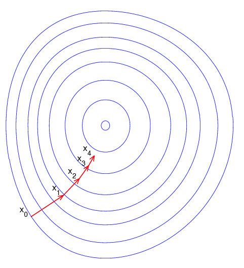
Preconditioning here can be viewed as changing the geometry of the vector space with the goal to make the level sets look like circles. In this case the preconditioned gradient aims closer to the point of the extrema as on the figure, which speeds up the convergence.

Connection to linear systems

The minimum of a quadratic function

where x and b are real column-vectors and A is a real symmetric positive-definite matrix, is exactly the solution of the linear equation A x = b . Since ∇ F ( x ) = A x − b , the preconditioned gradient descent method of minimizing F ( x ) is

This is the preconditioned Richardson iteration for solving a system of linear equations.

Connection to eigenvalue problems

The minimum of the Rayleigh quotient

where x is a real non-zero column-vector and A is a real symmetric positive-definite matrix, is the smallest eigenvalue of A , while the minimizer is the corresponding eigenvector. Since ∇ ρ ( x ) is proportional to A x − ρ ( x ) x , the preconditioned gradient descent method of minimizing ρ ( x ) is

This is an analog of preconditioned Richardson iteration for solving eigenvalue problems.

Variable preconditioning

In many cases, it may be beneficial to change the preconditioner at some or even every step of an iterative algorithm in order to accommodate for a changing shape of the level sets, as in

One should have in mind, however, that constructing an efficient preconditioner is very often computationally expensive. The increased cost of updating the preconditioner can easily override the positive effect of faster convergence.