Prandtl–Glauert transformation

Mathematical formulation

Inviscid compressible flow over slender bodies is governed by linearized compressible small-disturbance potential equation:

ϕ x x + ϕ y y + ϕ z z = M ∞ 2 ϕ x x (in flowfield)

together with the small-disturbance flow-tangency boundary condition.

V ∞ n x + ϕ y n y + ϕ z n z = 0 (on body surface)

M ∞ is the freestream Mach number, and n x , n y , n z are the surface-normal vector components. The unknown variable is the perturbation potential ϕ ( x , y , z ) , and the total velocity is given by its gradient plus the freestream velocity V ∞ which is assumed here to be along x .

V → = ∇ ϕ + V ∞ x ^ = ( V ∞ + ϕ x ) x ^ + ϕ y y ^ + ϕ z z ^

The above formulation is valid only if the small-disturbance approximation applies ,

| ∇ ϕ | ≪ V ∞

and in addition that there is no transonic flow, approximately stated by the requirement that the local Mach number not exceed unity.

[ 1 + ( γ + 1 ) ϕ x V ∞ ] M ∞ 2 < 1

The Prandtl-Glauert (PG) transformation uses the Prandtl-Glauert Factor β ≡ 1 − M ∞ 2 . It consists of scaling down all y and z dimensions and angle of attack by the factor of β , and the potential by β 2 .

x ¯ = x y ¯ = β y z ¯ = β z α ¯ = β α ϕ ¯ = β 2 ϕ

The small-disturbance potential equation then transforms to the Laplace equation,

ϕ ¯ x ¯ x ¯ + ϕ ¯ y ¯ y ¯ + ϕ ¯ z ¯ z ¯ = 0 (in flowfield)

and the flow-tangency boundary condition retains the same form.

V ∞ n ¯ x ¯ + ϕ ¯ y ¯ n ¯ y ¯ + ϕ ¯ z ¯ n ¯ z ¯ = 0 (on body surface)

This is the incompressible potential-flow problem about the transformed geometry with surface normal vector components n ¯ x ¯ , n ¯ y ¯ , n ¯ z ¯ . It can be solved by incompressible methods, such as thin airfoil theory, vortex lattice methods, panel methods, etc. The result is the transformed perturbation potential ϕ ¯ or its gradient components ϕ ¯ x ¯ , ϕ ¯ y ¯ , ϕ ¯ z ¯ in the transformed space. The physical linearized pressure coefficient is then obtained by the inverse transformation

C p = − 2 ϕ x V ∞ = − 2 β 2 ϕ ¯ x ¯ V ∞

which is known as Göthert's Rule

Results

For two-dimensional flow, the net result is that the C p and also the lift and moment coefficients c l , c m are increased by the factor 1 / β over the incompressible-flow values:

where C p 0 , c l 0 , c m 0 are the incompressible-flow values. This 2D-only result is known as the Prandtl Rule.

For three-dimensional flows, these simple 1 / β scalings do NOT apply. Instead, it is necessary to scale the xyz geometry as given above, and use the Göthert's Rule to compute the C p and subsequently the forces and moments. No simple results are possible, except in special cases. For example, using Lifting-Line Theory for a flat elliptical wing, the lift coefficient is

where AR is the wing's aspect ratio. Note that in the 2D case where AR → ∞ this reduces to the 2D case, since in incompressible 2D flow for a flat airfoil we have c l 0 = 2 π α , as given by Thin airfoil theory.

Limitations

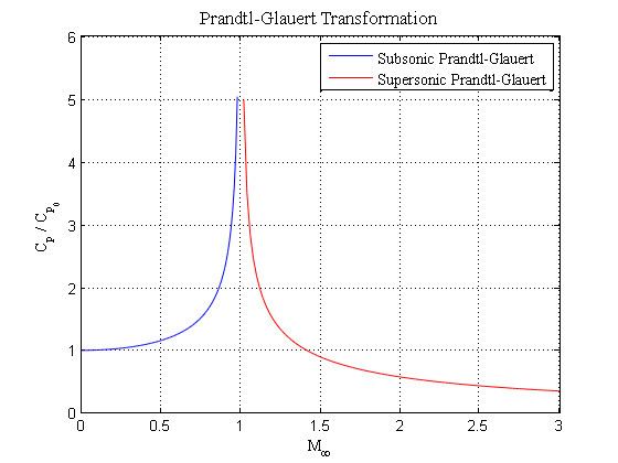
The PG transformation works well for all freestream Mach numbers up to 0.7 or so, or once transonic flow starts to appear.

History

Ludwig Prandtl had been teaching this transformation in his lectures for a while, however the first publication was in 1928 by Hermann Glauert. The introduction of this relation allowed the design of aircraft which were able to operate in higher subsonic speed areas. Originally all these results were developed for 2D flow. B.H. Göthert then pointed out that the geometry distortion of the PG transformation renders the simple 2D Prandtl Rule invalid for 3D, and properly stated the full 3D problem as described above.

The PG transformation was extended by Jakob Ackeret to supersonic-freestream flows. Like for the subsonic case, the supersonic case is valid only if there are no transonic effect, which requires that the body be slender and the freestream Mach is sufficiently far above unity.

Singularity

Near the sonic speed M ∞ ≃ 1 the PG transformation features a singularity. The singularity is also called the Prandtl–Glauert singularity, and the flow resistance is calculated to approach infinity. In reality, aerodynamic and thermodynamic perturbations get amplified strongly near the sonic speed, but a singularity does not occur. An explanation for this is that the linearized small-disturbance potential equation above is not valid, since it assumes that there are only small variations in Mach number within the flow and absence of compression shocks and thus is missing certain nonlinear terms. However, these become relevant as soon as any part of the flow field accelerates above the speed of sound, and become essential near M ∞ ≃ 1 . The more correct nonlinear equation does not exhibit the singularity.