
 | ||
The Prandtl lifting-line theory is a mathematical model that predicts lift distribution over a three-dimensional wing based on its geometry. It is also known as the Lanchester–Prandtl wing theory.
Contents
- Introduction
- Principle
- Derivation
- Lift and drag from coefficients
- Symmetric wing
- Rolling wings
- Control deflection
- Elliptical wings
- Useful approximations
- Limitations of the theory
- References
The theory was expressed independently by Frederick W. Lanchester in 1907, and by Ludwig Prandtl in 1918–1919 after working with Albert Betz and Max Munk.
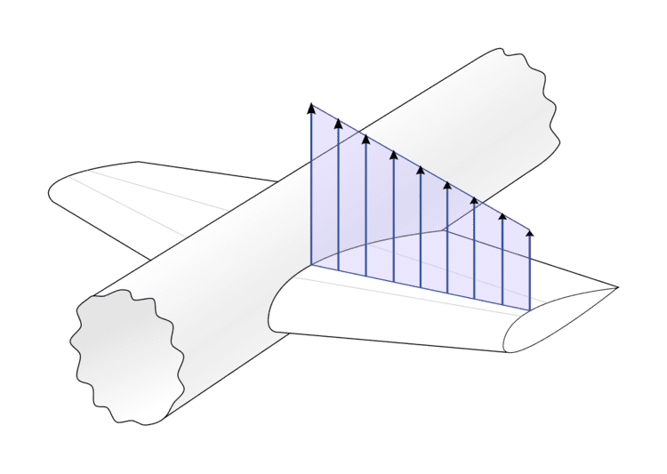
In this model, the vortex loses strength along the whole wingspan because it is shed as a vortex-sheet from the trailing edge, rather than just at the wing-tips.
Introduction
On a three-dimensional, finite wing, lift over each wing segment (local lift per unit span,
As such, it is difficult to predict analytically the overall amount of lift that a wing of given geometry will generate. The lifting-line theory yields the lift distribution along the span-wise direction,
Principle
The lifting-line theory applies the concept of circulation and the Kutta–Joukowski theorem,
so that instead of the lift distribution function, the unknown effectively becomes the distribution of circulation over the span,
Modeling the (unknown and sought-after) local lift with the (also unknown) local circulation allows us to account for the influence of one section over its neighbors. In this view, any span-wise change in lift is equivalent to a span-wise change of circulation. According to the Helmholtz theorems, a vortex filament cannot begin or terminate in the air. As such, any span-wise change in lift can be modeled as the shedding of a vortex filament down the flow, behind the wing.
This shed vortex, whose strength is the derivative of the (unknown) local wing circulation distribution,
This sideways influence (upwash on the outboard, downwash on the inboard) is the key to the lifting-line theory. Now, if the change in lift distribution is known at given lift section, it is possible to predict how that section influences the lift over its neighbors: the vertical induced velocity (upwash or downwash,
In mathematical terms, the local induced change of angle of attack
This leads to an integro-differential equation in the form of
Derivation
(Based on.)
Nomenclature:
The following are all functions of the wings span-wise station
To derive the model we start with the assumption that the circulation of the wing varies as a function of the spanwise locations. The function assumed is a Fourier function. Firstly, the coordinate for the spanwise location
and so the circulation is assumed to be:
Since the circulation of a section is related the
but since the coefficient of lift is a function of angle of attack:
hence the vortex strength at any particular spanwise station can be given by the equations:
This one equation has two unknowns: the value for
Differential element of circulation:
Differential downwash due to the differential element of circulation (acts like half an infinite vortex line):
The integral equation over the span of the wing to determine the downwash at a particular location is:
After appropriate substitutions and integrations we get:
And so the change in angle attack is determined by (assuming small angles):
By substituting equations 8 and 9 into RHS of equation 4 and equation 1 into the LHS of equation 4, we then get:
After rearranging, we get the series of simultaneous equations:
By taking a finite number of terms, equation 11 can be expressed in matrix form and solved for coefficients A. Note the left-hand side of the equation represents each element in the matrix, and the terms on the RHS of equation 11 represent the RHS of the matrix form. Each row in the matrix form represents a different span-wise station, and each column represents a different value for n.
Appropriate choices for
Lift and drag from coefficients
The lift can be determined by integrating the circulation terms:
which can be reduced to:
where
The induced drag can be determined from
or
where
Symmetric wing
For a symmetric wing, the even terms of the series coefficients are identically equal to 0, and so can be dropped.
Rolling wings
When the aircraft is rolling, an additional term can be added that adds the wing station distance multiplied by the rate of roll to give additional angle of attack change. Equation 3 then becomes:
where
Note that y can be negative, which introduces non-zero even coefficients in the equation that must be accounted for.
Control deflection
The effect of ailerons can be accounted for simply changing
Elliptical wings
For an elliptical wing with no twist, with:
The chord length is given as a function of span location as:
Also,
This yields the famous equation for the elliptic induced drag coefficient:
where
Useful approximations
A useful approximation is that
where
The theoretical value for
Lifting-line theory also states an equation for induced drag:.
where
Limitations of the theory
The lifting line theory does not take into account the following: