
 | ||
Overlap–save is the traditional name for an efficient way to evaluate the discrete convolution between a very long signal
Contents
where h[m]=0 for m outside the region [1, M].
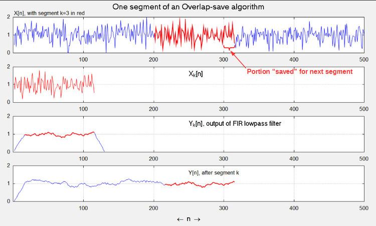
The concept is to compute short segments of y[n] of an arbitrary length L, and concatenate the segments together. Consider a segment that begins at n = kL + M, for any integer k, and define:
Then, for kL + M ≤ n ≤ kL + L + M − 1, and equivalently M ≤ n − kL ≤ L + M − 1, we can write:
The task is thereby reduced to computing yk[n], for M ≤ n ≤ L + M − 1. The process described above is illustrated in the accompanying figure.
Now note that if we periodically extend xk[n] with period N ≥ L + M − 1, according to:
the convolutions
The advantage is that the circular convolution can be computed very efficiently as follows, according to the circular convolution theorem:
where:
Pseudocode
(Overlap–save algorithm for linear convolution) h = FIR_impulse_response M = length(h) overlap = M-1 N = 4*overlap (or a nearby power-of-2) step_size = N-overlap H = DFT(h, N) position = 0 while position+N <= length(x) yt = IDFT( DFT( x(1+position : N+position), N ) * H, N ) y(1+position : step_size+position) = yt(M : N) #discard M-1 y-values position = position + step_size endEfficiency
When the DFT and its inverse is implemented by the FFT algorithm, the pseudocode above requires about N log2(N) + N complex multiplications for the FFT, product of arrays, and IFFT. Each iteration produces N-M+1 output samples, so the number of complex multiplications per output sample is about:
For example, when M=201 and N=1024, Eq.2 equals 13.67, whereas direct evaluation of Eq.1 would require up to 201 complex multiplications per output sample, the worst case being when both x and h are complex-valued. Also note that for any given M, Eq.2 has a minimum with respect to N. It diverges for both small and large block sizes.
Overlap–discard
Overlap–discard and Overlap–scrap are less commonly used labels for the same method described here. However, these labels are actually better (than overlap–save) to distinguish from overlap–add, because both methods "save", but only one discards. "Save" merely refers to the fact that M − 1 input (or output) samples from segment k are needed to process segment k + 1.
Extending overlap–save
The overlap-save algorithm may be extended to include other common operations of a system: