In signal processing, the overlap–add method (OA, OLA) is an efficient way to evaluate the discrete convolution of a very long signal
x
[
n
]
with a finite impulse response (FIR) filter
h
[
n
]
:
y
[
n
]
=
x
[
n
]
∗
h
[
n
]
=
d
e
f
∑
m
=
−
∞
∞
h
[
m
]
⋅
x
[
n
−
m
]
=
∑
m
=
1
M
h
[
m
]
⋅
x
[
n
−
m
]
,
where h[m] = 0 for m outside the region [1, M].
The concept is to divide the problem into multiple convolutions of h[n] with short segments of
x
[
n
]
:
x
k
[
n
]
=
d
e
f
{
x
[
n
+
k
L
]
n
=
1
,
2
,
…
,
L
0
otherwise
,
where L is an arbitrary segment length. Then:
x
[
n
]
=
∑
k
x
k
[
n
−
k
L
]
,
and y[n] can be written as a sum of short convolutions:
y
[
n
]
=
(
∑
k
x
k
[
n
−
k
L
]
)
∗
h
[
n
]
=
∑
k
(
x
k
[
n
−
k
L
]
∗
h
[
n
]
)
=
∑
k
y
k
[
n
−
k
L
]
,
where
y
k
[
n
]
=
d
e
f
x
k
[
n
]
∗
h
[
n
]
is zero outside the region [1, L + M − 1]. And for any parameter
N
≥
L
+
M
−
1
,
it is equivalent to the
N
-point circular convolution of
x
k
[
n
]
with
h
[
n
]
in the region [1, N].
The advantage is that the circular convolution can be computed very efficiently as follows, according to the circular convolution theorem:
where FFT and IFFT refer to the fast Fourier transform and inverse fast Fourier transform, respectively, evaluated over
N
discrete points.
Fig. 1 sketches the idea of the overlap–add method. The signal
x
[
n
]
is first partitioned into non-overlapping sequences, then the discrete Fourier transforms of the sequences
y
k
[
n
]
are evaluated by multiplying the FFT of
x
k
[
n
]
with the FFT of
h
[
n
]
. After recovering of
y
k
[
n
]
by inverse FFT, the resulting output signal is reconstructed by overlapping and adding the
y
k
[
n
]
as shown in the figure. The overlap arises from the fact that a linear convolution is always longer than the original sequences. In the early days of development of the fast Fourier transform,
L
was often chosen to be a power of 2 for efficiency, but further development has revealed efficient transforms for larger prime factorizations of L, reducing computational sensitivity to this parameter. A pseudocode of the algorithm is the following:
Algorithm 1 (
OA for linear convolution)
Evaluate the best value of N and L (L>0, N = M+L-1 nearest to power of 2).
Nx = length(x);
H = FFT(h,N)
(zero-padded FFT)
i = 1
y = zeros(1, M+Nx-1)
while i <= Nx
(Nx: the last index of x[n])
il = min(i+L-1,Nx)
yt = IFFT( FFT(x(i:il),N) * H, N)
k = min(i+N-1,M+Nx-1)
y(i:k) = y(i:k) + yt(1:k-i+1)
(add the overlapped output blocks)
i = i+L
end
This algorithm is based on the linearity of the DFT
When sequence x[n] is periodic, and Nx is the period, then y[n] is also periodic, with the same period. To compute one period of y[n], Algorithm 1 can first be used to convolve h[n] with just one period of x[n]. In the region M ≤ n ≤ Nx, the resultant y[n] sequence is correct. And if the next M − 1 values are added to the first M − 1 values, then the region 1 ≤ n ≤ Nx will represent the desired convolution. The modified pseudocode is:
Algorithm 2 (
OA for circular convolution)
Evaluate Algorithm 1
y(1:M-1) = y(1:M-1) + y(Nx+1:Nx+M-1)
y = y(1:Nx)
end
The cost of the convolution can be associated to the number of complex multiplications involved in the operation. The major computational effort is due to the FFT operation, which for a radix-2 algorithm applied to a signal of length
N
roughly calls for
C
=
N
2
log
2
N
complex multiplications. It turns out that the number of complex multiplications of the overlap-add method are:
C
O
A
=
⌈
N
x
N
−
M
+
1
⌉
N
(
log
2
N
+
1
)
C
O
A
accounts for the FFT+filter multiplication+IFFT operation.
The additional cost of the
M
L
sections involved in the circular version of the overlap–add method is usually very small and can be neglected for the sake of simplicity. The best value of
N
can be found by numerical search of the minimum of
C
O
A
(
N
)
=
C
O
A
(
2
m
)
by spanning the integer
m
in the range
log
2
(
M
)
≤
m
≤
log
2
(
N
x
)
. Being
N
a power of two, the FFTs of the overlap–add method are computed efficiently. Once evaluated the value of
N
it turns out that the optimal partitioning of
x
[
n
]
has
L
=
N
−
M
+
1
. For comparison, the cost of the standard circular convolution of
x
[
n
]
and
h
[
n
]
is:
C
S
=
N
x
(
log
2
N
x
+
1
)
Hence the cost of the overlap–add method scales almost as
O
(
N
x
log
2
N
)
while the cost of the standard circular convolution method is almost
O
(
N
x
log
2
N
x
)
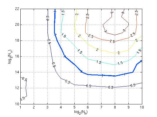
. However such functions accounts only for the cost of the complex multiplications, regardless of the other operations involved in the algorithm. A direct measure of the computational time required by the algorithms is of much interest. Fig. 2 shows the ratio of the measured time to evaluate a standard circular convolution using Eq.1 with the time elapsed by the same convolution using the overlap–add method in the form of Alg 2, vs. the sequence and the filter length. Both algorithms have been implemented under Matlab. The bold line represent the boundary of the region where the overlap–add method is faster (ratio>1) than the standard circular convolution. Note that the overlap–add method in the tested cases can be three times faster than the standard method.