Puneet Varma (Editor)

Milstein method

Updated on
Edit
Like
Comment
Share on FacebookTweet on TwitterShare on LinkedInShare on Reddit
Milstein method

In mathematics, the Milstein method is a technique for the approximate numerical solution of a stochastic differential equation. It is named after Grigori N. Milstein who first published the method in 1974.

Contents

Description

Consider the autonomous Itō stochastic differential equation

d X t = a ( X t ) d t + b ( X t ) d W t ,

with initial condition X0 = x0, where Wt stands for the Wiener process, and suppose that we wish to solve this SDE on some interval of time [0, T]. Then the Milstein approximation to the true solution X is the Markov chain Y defined as follows:

  • partition the interval [0, T] into N equal subintervals of width Δ t > 0 :
  • 0 = τ 0 < τ 1 < < τ N = T  with  τ n := n Δ t  and  Δ t = T N ;
  • set Y 0 = x 0 ;
  • recursively define Y n for 1 n N by
  • Y n + 1 = Y n + a ( Y n ) Δ t + b ( Y n ) Δ W n + 1 2 b ( Y n ) b ( Y n ) ( ( Δ W n ) 2 Δ t ) ,

    where b denotes the derivative of b ( x ) with respect to x and

    Δ W n = W τ n + 1 W τ n

    are independent and identically distributed normal random variables with expected value zero and variance Δ t . Then Y n will approximate X τ n for 0 n N , and increasing N will yield a better approximation.

    Note that when b ( Y n ) = 0 , i.e. the diffusion term does not depend on X t , this method is equivalent to the Euler–Maruyama method

    The Milstein scheme has both weak and strong order of convergence, Δ t , which is superior to the Euler–Maruyama method, which in turn has the same weak order of convergence, Δ t , but inferior strong order of convergence, Δ t .

    Intuitive derivation

    For this derivation, we will only look at geometric Brownian motion (GBM), the stochastic differential equation of which is given by

    d X t = μ X d t + σ X d W t

    with real constants μ and σ . Using Itō's lemma we get

    d ln X t = ( μ 1 2 σ 2 ) d t + σ d W t ,

    Thus, the solution to the GBM SDE is

    X t + Δ t = X t exp { t t + Δ t ( μ 1 2 σ 2 ) d t + t t + Δ t σ d W u } X t ( 1 + μ Δ t 1 2 σ 2 Δ t + σ Δ W t + 1 2 σ 2 ( Δ W t ) 2 ) = X t + a ( X t ) Δ t + b ( X t ) Δ W t + 1 2 b ( X t ) b ( X t ) ( ( Δ W t ) 2 Δ t )

    where

    a ( x ) = μ x ,   b ( x ) = σ x .

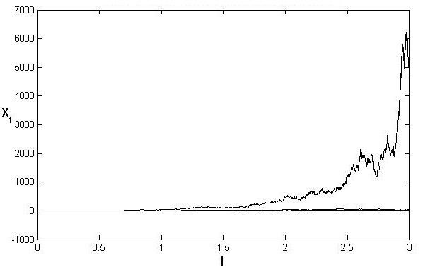
    See numerical solution is presented above for three different trajectories.

    References

    Milstein method Wikipedia