Microcanonical ensemble

Applicability

The microcanonical ensemble is sometimes considered to be the fundamental distribution of statistical thermodynamics, as its form can be justified on elementary grounds such as the principle of indifference: the microcanonical ensemble describes the possible states of an isolated mechanical system when the energy is known exactly, but without any more information about the internal state. Also, in some special systems the evolution is ergodic in which case the microcanonical ensemble is equal to the time-ensemble when starting out with a single state of energy E (a time-ensemble is the ensemble formed of all future states evolved from a single initial state).

In practice, the microcanonical ensemble does not correspond to an experimentally realistic situation. With a real physical system there is at least some uncertainty in energy, due to uncontrolled factors in the preparation of the system. Besides the difficulty of finding an experimental analogue, it is difficult to carry out calculations that satisfy exactly the requirement of fixed energy since it prevents logically independent parts of the system from being analyzed separately. Moreover there are ambiguities regarding the appropriate definitions of quantities such as entropy and temperature in the microcanonical ensemble.

Systems in thermal equilibrium with their environment have uncertainty in energy, and are instead described by the canonical ensemble or the grand canonical ensemble, the latter if the system is also in equilibrium with its environment in respect to particle exchange.

Thermodynamic analogies

Early work in statistical mechanics by Ludwig Boltzmann led to his eponymous entropy equation for a system of a given total energy, S = k log W, where W is the number of distinct states accessible by the system at that energy. Boltzmann did not elaborate too deeply on what exactly constitutes the set of distinct states of a system, besides the special case of an ideal gas. This topic was investigated to completion by Josiah Willard Gibbs who developed the generalized statistical mechanics for arbitrary mechanical systems, and defined the microcanonical ensemble described in this article. Gibbs investigated carefully the analogies between the microcanonical ensemble and thermodynamics, especially how they break down in the case of systems of few degrees of freedom. He introduced two further definitions of microcanonical entropy that do not depend on ω - the volume and surface entropy described above. (Note that the surface entropy differs from the Boltzmann entropy only by an ω-dependent offset.)

The volume entropy S_v and associated T_v form a close analogy to thermodynamic entropy and temperature. It is possible to show exactly that

(⟨P⟩ is the ensemble average pressure) as expected for the first law of thermodynamics. A similar equation can be found for the surface (Boltzmann) entropy and its associated T_s, however the "pressure" in this equation is a complicated quantity unrelated to the average pressure.

The microcanonical T_v and T_s are not entirely satisfactory in their analogy to temperature. Outside of the thermodynamic limit, a number of artifacts occur.

The preferred solution to these problems is avoid use of the microcanonical ensemble. In many realistic cases a system is thermostatted to a heat bath so that the energy is not precisely known. Then, a more accurate description is the canonical ensemble or grand canonical ensemble, both of which have complete correspondence to thermodynamics.

Precise expressions for the ensemble

The precise mathematical expression for a statistical ensemble depends on the kind of mechanics under consideration—quantum or classical—since the notion of a "microstate" is considerably different in these two cases. In quantum mechanics, diagonalization provides a discrete set of microstates with specific energies. The classical mechanical case involves instead an integral over canonical phase space, and the size of microstates in phase space can be chosen somewhat arbitrarily.

To construct the microcanonical ensemble, it is necessary in both types of mechanics to first specify a range of energy. In the expressions below the function f ( H − E ω ) (a function of H, peaking at E with width ω) will be used to represent the range of energy in which to include states. An example of this function would be

or, more smoothly,

Quantum mechanical

A statistical ensemble in quantum mechanics is represented by a density matrix, denoted by ρ̂. The microcanonical ensemble can be written using bra–ket notation, in terms of the system's energy eigenstates and energy eigenvalues. Given a complete basis of energy eigenstates |ψ_i⟩, indexed by i, the microcanonical ensemble is:

where the H_i are the energy eigenvalues determined by Ĥ|ψ_i⟩ = H_i|ψ_i⟩ (here Ĥ is the system's total energy operator, i. e., Hamiltonian operator). The value of W is determined by demanding that ρ̂ is a normalized density matrix, and so

The state volume function (used to calculate entropy) is given by

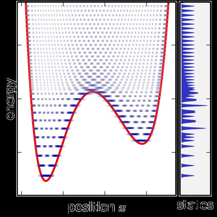
The microcanonical ensemble is defined by taking the limit of the density matrix as the energy width goes to zero, however a problematic situation occurs once the energy width becomes smaller than the spacing between energy levels. For very small energy width, the ensemble does not exist at all for most values of E since no states fall within the range. When the ensemble does exist it typically only contains one (or two) states, since in a complex system the energy levels are only ever equal by accident (see random matrix theory for more discussion on this point). Moreover, the state volume function also increases only in discrete increments and so its derivative is only ever infinite or zero, making it difficult to define the density of states. This problem can be solved by not taking the energy range completely to zero and smoothing the state volume function, however this makes the definition of the ensemble more complicated since it becomes then necessary to specify the energy range in addition to other variables (together, an NVEω ensemble).

Classical mechanical

In classical mechanics, an ensemble is represented by a joint probability density function ρ(p₁, … p_n, q₁, … q_n) defined over the system's phase space. The phase space has n generalized coordinates called q₁, … q_n, and n associated canonical momenta called p₁, … p_n.

The probability density function for the microcanonical ensemble is:

where

Again, the value of W is determined by demanding that ρ is a normalized probability density function:

This integral is taken over the entire phase space. The state volume function (used to calculate entropy) is defined by

As the energy width ω is taken to zero, the value of W decreases in proportion to ω as W = ω (dv/dE).

Based on the above definition, the microcanonical ensemble can be visualized as an infinitesimally thin shell in phase space, centered on a constant-energy surface. Although the microcanonical ensemble is confined to this surface, it is not necessarily uniformly distributed over that surface: if the gradient of energy in phase space varies, then the microcanonical ensemble is "thicker" (more concentrated) in some parts of the surface than others. This feature is an unavoidable consequence of requiring that the microcanonical ensemble is a steady-state ensemble.