Macroscopic quantum phenomena

Consequences of the macroscopic occupation

The concept of macroscopically-occupied quantum states is introduced by Fritz London. In this section it will be explained what it means if the ground state is occupied by a very large number of particles. We start with the wave function of the ground state written as

with Ψ₀ the amplitude and φ the phase. The wave function is normalized so that

The physical interpretation of the quantity

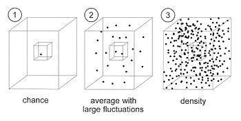
depends on the number of particles. Fig.1 represents a container with a certain number of particles with a small control volume ΔV inside. We check from time to time how many particles are in the control box. We distinguish three cases:

1. There is only one particle. In this case the control volume is empty most of the time. However, there is a certain chance to find the particle in it given by Eq.(3). The chance is proportional to ΔV. The factor ΨΨ^∗ is called the chance density.

2. If the number of particles is a bit larger there are usually some particles inside the box. We can define an average, but the actual number of particles in the box has relatively large fluctuations around this average.

3. In the case of a very large number of particles there will always be a lot of particles in the small box. The number will fluctuate but the fluctuations around the average are relatively small. The average number is proportional to ΔV and ΨΨ^∗ is now interpreted as the particle density.

In quantum mechanics the particle probability flow density J_p (unit: particles per second per m²) can be derived from the Schrödinger equation to be

with q the charge of the particle and A → the vector potential. With Eq.(1)

If the wave function is macroscopically occupied the particle probability flow density becomes a particle flow density. We introduce the fluid velocity v_s via the mass flow density

The density (mass per m³) is

so Eq.(5) results in

This important relation connects the velocity, a classical concept, of the condensate with the phase of the wave function, a quantum-mechanical concept.

Superfluidity

Below the lambda-temperature, helium shows the unique property of superfluidity. The fraction of the liquid that forms the superfluid component is a macroscopic quantum fluid. The helium atom is a neutral particle, so q=0. Furthermore, when considering helium-4, the relevant particle mass is m=m₄, so Eq.(8) reduces to

For an arbitrary loop in the liquid, this gives

Due to the single-valued nature of the wave function

with n integer, we have

The quantity

is the quantum of circulation. For a circular motion with radius r

In case of a single quantum (n=1)

When superfluid helium is put in rotation, Eq.(13) will not be satisfied for all loops inside the liquid unless the rotation is organized around vortex lines (as depicted in Fig.2). These lines have a vacuum core with a diameter of about 1 Å (which is smaller than the average particle distance). The superfluid helium rotates around the core with very high speeds. Just outside the core (r = 1 Å), the velocity is as large as 160 m/s. The cores of the vortex lines and the container rotate as a solid body around the rotation axes with the same angular velocity. The number of vortex lines increases with the angular velocity (as shown in the upper half of the figure). Note that the two right figures both contain six vortex lines, but the lines are organized in different stable patterns.

Superconductivity

In the original paper Ginzburg and Landau observed the existence of two types of superconductors depending on the energy of the interface between the normal and superconducting states.The Meissner state breaks down when the applied magnetic field is too large. Superconductors can be divided into two classes according to how this breakdown occurs. In Type I superconductors, superconductivity is abruptly destroyed when the strength of the applied field rises above a critical value H_c. Depending on the geometry of the sample, one may obtain an intermediate state consisting of a baroque pattern of regions of normal material carrying a magnetic field mixed with regions of superconducting material containing no field. In Type II superconductors, raising the applied field past a critical value H_c1 leads to a mixed state (also known as the vortex state) in which an increasing amount of magnetic flux penetrates the material, but there remains no resistance to the flow of electric current as long as the current is not too large. At a second critical field strength H_c2, superconductivity is destroyed. The mixed state is actually caused by vortices in the electronic superfluid, sometimes called fluxons because the flux carried by these vortices is quantized. Most pure elemental superconductors, except niobium and carbon nanotubes, are Type I, while almost all impure and compound superconductors are Type II.

The most important finding from Ginzburg–Landau theory was made by Alexei Abrikosov in 1957. He used Ginzburg–Landau theory to explain experiments on superconducting alloys and thin films. He found that in a type-II superconductor in a high magnetic field, the field penetrates in a triangular lattice of quantized tubes of flux vortices.

Fluxoid quantization

For superconductors the bosons involved are the so-called Cooper pairs which are quasiparticles formed by two electrons. Hence m = 2m_e and q = -2e where m_e and e are the mass of an electron and the elementary charge. It follows from Eq.(8) that

Integrating Eq.(15) over a closed loop gives

As in the case of helium we define the vortex strength

and use the general relation

where Φ is the magnetic flux enclosed by the loop. The so-called fluxoid is defined by

In general the values of κ and Φ depend on the choice of the loop. Due to the single-valued nature of the wave function and Eq.(16) the fluxoid is quantized

The unit of quantization is called the flux quantum

The flux quantum plays a very important role in superconductivity. The earth magnetic field is very small (about 50 μT), but it generates one flux quantum in an area of 6 by 6 μm. So, the flux quantum is very small. Yet it was measured to an accuracy of 9 digits as shown in Eq.(21). Nowadays the value given by Eq.(21) is exact by definition.

In Fig. 3 two situations are depicted of superconducting rings in an external magnetic field. One case is a thick-walled ring and in the other case the ring is also thick-walled, but is interrupted by a weak link. In the latter case we will meet the famous Josephson relations. In both cases we consider a loop inside the material. In general a superconducting circulation current will flow in the material. The total magnetic flux in the loop is the sum of the applied flux Φ_a and the self-induced flux Φ_s induced by the circulation current

Thick ring

The first case is a thick ring in an external magnetic field (Fig. 3a). The currents in a superconductor only flow in a thin layer at the surface. The thickness of this layer is determined by the so-called London penetration depth. It is of μm size or less. We consider a loop far away from the surface so that v_s=0 everywhere so κ=0. In that case the fluxoid is equal to the magnetic flux (Φ_v=Φ). If v_s=0 Eq.(15) reduces to

Taking the rotation gives

Using the well-known relations ∇ → × ∇ → φ = 0 and ∇ → × A → = B → shows that the magnetic field in the bulk of the superconductor is zero as well. So, for thick rings, the total magnetic flux in the loop is quantized according to

Interrupted ring, weak links

Weak links play a very important role in modern superconductivity. In most cases weak links are oxide barriers between two superconducting thin films, but it can also be a crystal boundary (in the case of high-Tc superconductors). A schematic representation is given in Fig. 4. Now consider the ring which is thick everywhere except for a small section where the ring is closed via a weak link (Fig. 3b). The velocity is zero except near the weak link. In these regions the velocity contribution to the total phase change in the loop is given by (with Eq.(15))

The line integral is over the contact from one side to the other in such a way that the end points of the line are well inside the bulk of the superconductor where v_s=0. So the value of the line integral is well-defined (e.g. independent of the choice of the end points). With Eqs.(19), (22), and (26)

Without proof we state that the supercurrent through the weak link is given by the so-called DC Josephson relation

The voltage over the contact is given by the AC Josephson relation

The names of these relations (DC and AC relations) are misleading since they both hold in DC and AC situations. In the steady state (constant Δ φ ∗ ) Eq.(29) shows that V=0 while a nonzero current flows through the junction. In the case of a constant applied voltage (voltage bias) Eq.(29) can be integrated easily and gives

Substitution in Eq.(28) gives

This is an AC current. The frequency

is called the Josephson frequency. One μV gives a frequency of about 500 MHz. By using Eq.(32) the flux quantum is determined with the high precision as given in Eq.(21).

The energy difference of a Cooper pair, moving from one side of the contact to the other, is ΔE = 2eV. With this expression Eq.(32) can be written as ΔE = hν which is the relation for the energy of a photon with frequency ν.

The AC Josephson relation (Eq.(29)) can be easily understood in terms of Newton's law, (or from one of the London equation's). We start with Newton's law Substituting the expression for the Lorentz force and using the general expression for the co-moving time derivative gives Eq.(8) gives so Take the line integral of this expression. In the end points the velocities are zero so the ∇v² term gives no contribution. Using and Eq.(26), with q = -2e and m =2m_e, gives Eq.(29).

DC SQUID

Figure 5 shows a so-called DC SQUID. It consists of two superconductors connected by two weak links. The fluxoid quantization of a loop through the two bulk superconductors and the two weak links demands

If the self-inductance of the loop can be neglected the magnetic flux in the loop Φ is equal to the applied flux

with B the magnetic field, applied perpendicular to the surface, and A the surface area of the loop. The total supercurrent is given by

Substitution of Eq(33) in (35) gives

Using a well known geometrical formula we get

Since the sin-function can vary only between −1 and +1 a steady solution is only possible if the applied current is below a critical current given by

Note that the critical current is periodic in the applied flux with period Φ₀. The dependence of the critical current on the applied flux is depicted in Fig. 6. It has a strong resemblance with the interference pattern generated by a laser beam behind a double slit. In practice the critical current is not zero at half integer values of the flux quantum of the applied flux. This is due to the fact that the self-inductance of the loop cannot be neglected.

Type II superconductivity

Type-II superconductivity is characterized by two critical fields called B_c1 and B_c2. At a magnetic field B_c1 the applied magnetic field starts to penetrate the sample, but the sample is still superconducting. Only at a field of B_c2 the sample is completely normal. For fields in between B_c1 and B_c2 magnetic flux penetrates the superconductor in well-organized patterns, the so-called Abrikosov vortex lattice similar to the pattern shown in Fig. 2. A cross section of the superconducting plate is given in Fig. 7. Far away from the plate the field is homogeneous, but in the material superconducting currents flow which squeeze the field in bundles of exactly one flux quantum. The typical field in the core is as big as 1 tesla. The currents around the vortex core flow in a layer of about 50 nm with current densities on the order of 15×10¹² A/m². That corresponds with 15 million ampère in a wire of one mm².

Dilute quantum gases

The classical types of quantum systems, superconductors and superfluid helium, were discovered in the beginning of the 20th century. Near the end of the 20th century, scientists discovered how to create very dilute atomic or molecular gases, cooled first by laser cooling and then by evaporative cooling. They are trapped using magnetic fields or optical dipole potentials in ultrahigh vacuum chambers. Isotopes which have been used include rubidium (Rb-87 and Rb-85), strontium (Sr-87, Sr-86, and Sr-84) potassium (K-39 and K-40), sodium (Na-23), lithium (Li-7 and Li-6), and hydrogen (H-1). The temperatures to which they can be cooled are as low as a few nanokelvin. The developments have been very fast in the past few years. A team of NIST and the University of Colorado has succeeded in creating and observing vortex quantization in these systems. The concentration of vortices increases with the angular velocity of the rotation, similar to the case of superfluid helium and superconductivity.