Logit normal distribution - Alchetron, the free social encyclopedia

Support x ∈ (0, 1)		Mean no analytical solution

Notation P ( N ( μ , σ 2 ) ) {\displaystyle P({\mathcal {N}}(\mu ,\,\sigma ^{2}))} Parameters σ > 0 — squared scale (real),μ ∈ R — location PDF 1 σ 2 π e − ( logit ⁡ ( x ) − μ ) 2 2 σ 2 1 x ( 1 − x ) {\displaystyle {\frac {1}{\sigma {\sqrt {2\pi }}}}\,e^{-{\frac {(\operatorname {logit} (x)-\mu )^{2}}{2\sigma ^{2}}}}{\frac {1}{x(1-x)}}} CDF 1 2 [ 1 + erf ⁡ ( logit ⁡ ( x ) − μ 2 σ 2 ) ] {\displaystyle {\frac {1}{2}}{\Big [}1+\operatorname {erf} {\Big (}{\frac {\operatorname {logit} (x)-\mu }{\sqrt {2\sigma ^{2}}}}{\Big )}{\Big ]}}

In probability theory, a logit-normal distribution is a probability distribution of a random variable whose logit has a normal distribution. If Y is a random variable with a normal distribution, and P is the logistic function, then X = P(Y) has a logit-normal distribution; likewise, if X is logit-normally distributed, then Y = logit(X)= log (X/(1-X)) is normally distributed. It is also known as the logistic normal distribution, which often refers to a multinomial logit version (e.g.).

Probability density function

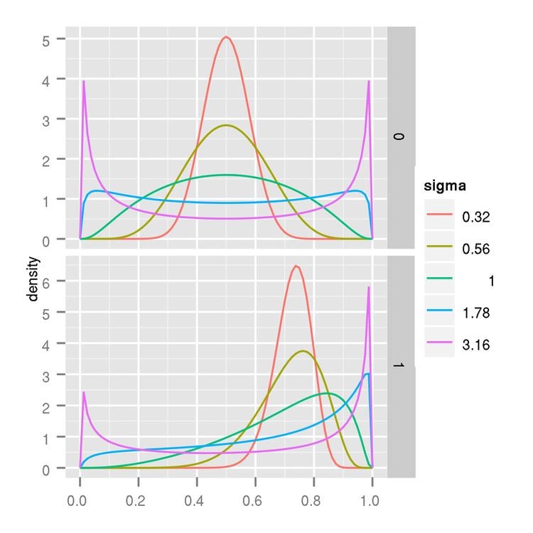
The probability density function (PDF) of a logit-normal distribution, for 0 ≤ x ≤ 1, is:

f X ( x ; μ , σ ) = 1 σ 2 π 1 x ( 1 − x ) e − ( logit ⁡ ( x ) − μ ) 2 2 σ 2

where μ and σ are the mean and standard deviation of the variable’s logit (by definition, the variable’s logit is normally distributed).

The density obtained by changing the sign of μ is symmetrical, in that it is equal to f(1-x;-μ,σ), shifting the mode to the other side of 0.5 (the midpoint of the (0,1) interval).

Moments

The moments of the logit-normal distribution have no analytic solution. However, they can be estimated by numerical integration.

Mode

When the derivative of the density equals 0 then the location of the mode x satisfies the following equation:

logit ⁡ ( x ) = σ 2 ( 2 x − 1 ) + μ .

Multivariate generalization

The logistic normal distribution is a generalization of the logit–normal distribution to D-dimensional probability vectors by taking a logistic transformation of a multivariate normal distribution.

Probability density function

The probability density function is:

f X ( x ; μ , Σ ) = 1 | 2 π Σ | 1 2 1 ∏ i = 1 D x i e − 1 2 { log ⁡ ( x − D x D ) − μ } ⊤ Σ − 1 { log ⁡ ( x − D x D ) − μ } , x ∈ S D ,

where x − D denotes a vector of the first (D-1) components of x and S D denotes the simplex of D-dimensional probability vectors. This follows from applying the additive logistic transformation to map a multivariate normal random variable y ∼ N ( μ , Σ ) , y ∈ R D − 1 to the simplex:

x = [ e y 1 1 + ∑ i = 1 D − 1 e y i , … , e y D − 1 1 + ∑ i = 1 D − 1 e y i , 1 1 + ∑ i = 1 D − 1 e y i ] ⊤

The unique inverse mapping is given by:

y = [ log ⁡ ( x 1 x D ) , … , log ⁡ ( x D − 1 x D ) ] ⊤ .

This is the case of a vector x which components sum up to one. In the case of x with sigmoidal elements, that is, when

y = [ log ⁡ ( x 1 1 − x 1 ) , … , log ⁡ ( x D 1 − x D ) ] ⊤

we have

f X ( x ; μ , Σ ) = 1 | 2 π Σ | 1 2 1 ∏ i = 1 D ( x i ( 1 − x i ) ) e − 1 2 { log ⁡ ( x 1 − x ) − μ } ⊤ Σ − 1 { log ⁡ ( x 1 − x ) − μ }

where the log and the division in the argument are taken element-wise. This is because the Jacobian matrix of the transformation is diagonal with elements 1 x i ( 1 − x i ) .

Use in statistical analysis

The logistic normal distribution is a more flexible alternative to the Dirichlet distribution in that it can capture correlations between components of probability vectors. It also has the potential to simplify statistical analyses of compositional data by allowing one to answer questions about log-ratios of the components of the data vectors. One is often interested in ratios rather than absolute component values.

The probability simplex is a bounded space, making standard techniques that are typically applied to vectors in R n less meaningful. Aitchison described the problem of spurious negative correlations when applying such methods directly to simplicial vectors. However, mapping compositional data in S D through the inverse of the additive logistic transformation yields real-valued data in R D − 1 . Standard techniques can be applied to this representation of the data. This approach justifies use of the logistic normal distribution, which can thus be regarded as the "Gaussian of the simplex".

Relationship with the Dirichlet distribution

The Dirichlet and logistic normal distributions are never exactly equal for any choice of parameters. However, Aitchison described a method for approximating a Dirichlet with a logistic normal such that their Kullback–Leibler divergence (KL) is minimized:

K ( p , q ) = ∫ S D p ( x | α ) log ⁡ ( p ( x | α ) q ( x | μ , Σ ) ) d x

This is minimized by:

μ ∗ = E p [ log ⁡ ( x − D x D ) ] , Σ ∗ = Var p [ log ⁡ ( x − D x D ) ]

Using moment properties of the Dirichlet distribution, the solution can be written in terms of the digamma ψ and trigamma ψ ′ functions:

μ i ∗ = ψ ( α i ) − ψ ( α D ) , i = 1 , ⋯ , D − 1 Σ i i ∗ = ψ ′ ( α i ) + ψ ′ ( α D ) , i = 1 , ⋯ , D − 1 Σ i j ∗ = ψ ′ ( α D ) , i ≠ j

This approximation is particularly accurate for large α . In fact, one can show that for α i → ∞ , i = 1 , ⋯ , D , we have that p ( x | α ) → q ( x | μ ∗ , Σ ∗ ) .

References

Logit-normal distribution Wikipedia

(Text) CC BY-SA

Contents

Probability density function

Moments

Mode

Multivariate generalization

Probability density function

Use in statistical analysis

Relationship with the Dirichlet distribution

References