
 | ||
In probability theory and information theory, the Kullback–Leibler divergence, also called information divergence, information gain, relative entropy, KLIC, or KL divergence, is a measure (but not a metric) of the non-symmetric difference between two probability distributions P and Q. The Kullback–Leibler divergence was originally introduced by Solomon Kullback and Richard Leibler in 1951 as the directed divergence between two distributions; Kullback himself preferred the name discrimination information. It is discussed in Kullback's historic text, Information Theory and Statistics.
Contents
- Definition
- Characterization
- Motivation
- Properties
- KullbackLeibler divergence for multivariate normal distributions
- Relation to metrics
- Fisher information metric
- Relation to other quantities of information theory
- KullbackLeibler divergence and Bayesian updating
- Bayesian experimental design
- Discrimination information
- Principle of minimum discrimination information
- Relationship to available work
- Quantum information theory
- Relationship between models and reality
- Symmetrised divergence
- Relationship to other probability distance measures
- Data differencing
- References
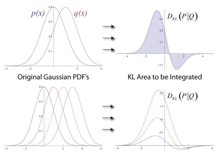
Expressed in the language of Bayesian inference, the Kullback–Leibler divergence from Q to P, denoted DKL(P‖Q), is a measure of the information gained when one revises one's beliefs from the prior probability distribution Q to the posterior probability distribution P. In other words, it is the amount of information lost when Q is used to approximate P. In applications, P typically represents the "true" distribution of data, observations, or a precisely calculated theoretical distribution, while Q typically represents a theory, model, description, or approximation of P.
The Kullback–Leibler divergence is a special case of a broader class of divergences called f-divergences as well as the class of Bregman divergences. It is the only such divergence over probabilities that is a member of both classes. Although it is often intuited as a way of measuring the distance between probability distributions, the Kullback–Leibler divergence is not a true metric. It does not obey the triangle inequality, and in general DKL(P‖Q) does not equal DKL(Q‖P). However, its infinitesimal form, specifically its Hessian, gives a metric tensor known as the Fisher information metric.
In the context of machine learning, the Kullback–Leibler divergence is often called the information gain achieved if P is used instead of Q. By analogy with information theory, it is also called the relative entropy of P with respect to Q. In the context of coding theory, Kullback–Leibler divergence can be construed as measure the expected number of extra bits required to code samples from P using a code optimized for Q rather than the code optimized for P.
Definition
For discrete probability distributions P and Q, the Kullback–Leibler divergence from Q to P is defined to be
In other words, it is the expectation of the logarithmic difference between the probabilities P and Q, where the expectation is taken using the probabilities P. The Kullback–Leibler divergence is defined only if Q(i)=0 implies P(i)=0, for all i (absolute continuity). Whenever P(i) is zero the contribution of the i-th term is interpreted as zero because
For distributions P and Q of a continuous random variable, the Kullback–Leibler divergence is defined to be the integral:
where p and q denote the densities of P and Q.
More generally, if P and Q are probability measures over a set X, and P is absolutely continuous with respect to Q, then the Kullback–Leibler divergence from Q to P is defined as
where
which we recognize as the entropy of P relative to Q. Continuing in this case, if
The logarithms in these formulae are taken to base 2 if information is measured in units of bits, or to base e if information is measured in nats. Most formulas involving the Kullback–Leibler divergence hold regardless of the base of the logarithm.
Various conventions exist for referring to DKL(P‖Q) in words. Often it is referred to as the divergence between P and Q; however this fails to convey the fundamental asymmetry in the relation. Sometimes, as in this article, it may be found described as the divergence of P from, or with respect to Q. This reflects the asymmetry in Bayesian inference, which starts from a prior Q and updates to the posterior P.
Characterization
Arthur Hobson proved that the Kullback–Leibler divergence is the only measure of difference between probability distributions that satisfies some desired properties, which are the canonical extension to those appearing in a commonly used characterization of entropy. Consequently, mutual information is the only measure of mutual dependence that obeys certain related conditions, since it can be defined in terms of Kullback-Leibler divergence.
There is also a Bayesian characterization of the Kullback–Leibler divergence.
Motivation
In information theory, the Kraft–McMillan theorem establishes that any directly decodable coding scheme for coding a message to identify one value xi out of a set of possibilities X can be seen as representing an implicit probability distribution q(xi)=2−li over X, where li is the length of the code for xi in bits. Therefore, the Kullback–Leibler divergence can be interpreted as the expected extra message-length per datum that must be communicated if a code that is optimal for a given (wrong) distribution Q is used, compared to using a code based on the true distribution P.
where H(P,Q) is the cross entropy of P and Q, and H(P) is the entropy of P.
Note also that there is a relation between the Kullback–Leibler divergence and the "rate function" in the theory of large deviations.
Properties
Kullback–Leibler divergence for multivariate normal distributions
Suppose that we have two multivariate normal distributions, with means
The logarithm in the last term must be taken to base e since all terms apart from the last are base-e logarithms of expressions that are either factors of the density function or otherwise arise naturally. The equation therefore gives a result measured in nats. Dividing the entire expression above by loge 2 yields the divergence in bits.
Relation to metrics
One might be tempted to call the Kullback–Leibler divergence a "distance metric" on the space of probability distributions, but this would not be correct as it is not symmetric – that is,
then it is said that
Pinsker's inequality entails that
where the latter stands for the usual convergence in total variation.
Following Rényi (1970, 1961)
Fisher information metric
However, the Kullback–Leibler divergence is rather directly related to a metric, specifically, the Fisher information metric. This can be made explicit as follows. Assume that the probability distributions P and Q are both parameterized by some (possibly multi-dimensional) parameter
with
and by the Taylor expansion one has up to second order
where the Hessian matrix of the divergence
must be positive semidefinite. Letting
Relation to other quantities of information theory
Many of the other quantities of information theory can be interpreted as applications of the Kullback–Leibler divergence to specific cases.
The self-information,
is the Kullback–Leibler divergence of the probability distribution P(i) from a Kronecker delta representing certainty that i = m — i.e. the number of extra bits that must be transmitted to identify i if only the probability distribution P(i) is available to the receiver, not the fact that i = m.
The mutual information,
is the Kullback–Leibler divergence of the product P(X)P(Y) of the two marginal probability distributions from the joint probability distribution P(X,Y) — i.e. the expected number of extra bits that must be transmitted to identify X and Y if they are coded using only their marginal distributions instead of the joint distribution. Equivalently, if the joint probability P(X,Y) is known, it is the expected number of extra bits that must on average be sent to identify Y if the value of X is not already known to the receiver.
The Shannon entropy,
is the number of bits which would have to be transmitted to identify X from N equally likely possibilities, less the Kullback–Leibler divergence of the uniform distribution PU(X) from the true distribution P(X) — i.e. less the expected number of bits saved, which would have had to be sent if the value of X were coded according to the uniform distribution PU(X) rather than the true distribution P(X).
The conditional entropy,
is the number of bits which would have to be transmitted to identify X from N equally likely possibilities, less the Kullback–Leibler divergence of the product distribution PU(X) P(Y) from the true joint distribution P(X,Y) — i.e. less the expected number of bits saved which would have had to be sent if the value of X were coded according to the uniform distribution PU(X) rather than the conditional distribution P(X | Y) of X given Y.
The cross entropy between two probability distributions measures the average number of bits needed to identify an event from a set of possibilities, if a coding scheme is used based on a given probability distribution
Kullback–Leibler divergence and Bayesian updating
In Bayesian statistics the Kullback–Leibler divergence can be used as a measure of the information gain in moving from a prior distribution to a posterior distribution:
This distribution has a new entropy:
...which may be less than or greater than the original entropy
to the message length. This therefore represents the amount of useful information, or information gain, about
If a further piece of data,
and so the combined information gain does not obey the triangle inequality:
All one can say is that on average, averaging using
Bayesian experimental design
A common goal in Bayesian experimental design is to maximise the expected Kullback–Leibler divergence between the prior and the posterior. When posteriors are approximated to be Gaussian distributions, a design maximising the expected Kullback–Leibler divergence is called Bayes d-optimal.
Discrimination information
The Kullback–Leibler divergence DKL( p(x|H1) ‖ p(x|H0) ) can also be interpreted as the expected discrimination information for H1 over H0: the mean information per sample for discriminating in favor of a hypothesis H1 against a hypothesis H0, when hypothesis H1 is true. Another name for this quantity, given to it by I.J. Good, is the expected weight of evidence for H1 over H0 to be expected from each sample.
The expected weight of evidence for H1 over H0 is not the same as the information gain expected per sample about the probability distribution p(H) of the hypotheses,
Either of the two quantities can be used as a utility function in Bayesian experimental design, to choose an optimal next question to investigate: but they will in general lead to rather different experimental strategies.
On the entropy scale of information gain there is very little difference between near certainty and absolute certainty—coding according to a near certainty requires hardly any more bits than coding according to an absolute certainty. On the other hand, on the logit scale implied by weight of evidence, the difference between the two is enormous – infinite perhaps; this might reflect the difference between being almost sure (on a probabilistic level) that, say, the Riemann hypothesis is correct, compared to being certain that it is correct because one has a mathematical proof. These two different scales of loss function for uncertainty are both useful, according to how well each reflects the particular circumstances of the problem in question.
Principle of minimum discrimination information
The idea of Kullback–Leibler divergence as discrimination information led Kullback to propose the Principle of Minimum Discrimination Information (MDI): given new facts, a new distribution f should be chosen which is as hard to discriminate from the original distribution f0 as possible; so that the new data produces as small an information gain DKL( f ‖ f0 ) as possible.
For example, if one had a prior distribution p(x,a) over x and a, and subsequently learnt the true distribution of a was u(a), the Kullback–Leibler divergence between the new joint distribution for x and a, q(x|a) u(a), and the earlier prior distribution would be:
i.e. the sum of the Kullback–Leibler divergence of p(a) the prior distribution for a from the updated distribution u(a), plus the expected value (using the probability distribution u(a)) of the Kullback–Leibler divergence of the prior conditional distribution p(x|a) from the new conditional distribution q(x|a). (Note that often the later expected value is called the conditional Kullback–Leibler divergence (or conditional relative entropy) and denoted by DKL(q(x|a)‖p(x|a))) This is minimized if q(x|a) = p(x|a) over the whole support of u(a); and we note that this result incorporates Bayes' theorem, if the new distribution u(a) is in fact a δ function representing certainty that a has one particular value.
MDI can be seen as an extension of Laplace's Principle of Insufficient Reason, and the Principle of Maximum Entropy of E.T. Jaynes. In particular, it is the natural extension of the principle of maximum entropy from discrete to continuous distributions, for which Shannon entropy ceases to be so useful (see differential entropy), but the Kullback–Leibler divergence continues to be just as relevant.
In the engineering literature, MDI is sometimes called the Principle of Minimum Cross-Entropy (MCE) or Minxent for short. Minimising the Kullback–Leibler divergence from m to p with respect to m is equivalent to minimizing the cross-entropy of p and m, since
which is appropriate if one is trying to choose an adequate approximation to p. However, this is just as often not the task one is trying to achieve. Instead, just as often it is m that is some fixed prior reference measure, and p that one is attempting to optimise by minimising DKL(p‖m) subject to some constraint. This has led to some ambiguity in the literature, with some authors attempting to resolve the inconsistency by redefining cross-entropy to be DKL(p‖m), rather than H(p,m).
Relationship to available work
Surprisals add where probabilities multiply. The surprisal for an event of probability
Best-guess states (e.g. for atoms in a gas) are inferred by maximizing the average surprisal
When temperature
More generally the work available relative to some ambient is obtained by multiplying ambient temperature
Quantum information theory
For density matrices P and Q on a Hilbert space, the K–L divergence (or quantum relative entropy as it is often called in this case) from Q to P is defined to be
In quantum information science the minimum of
Relationship between models and reality
Just as Kullback–Leibler divergence of "actual from ambient" measures thermodynamic availability, Kullback–Leibler divergence of "reality from a model" is also useful even if the only clues we have about reality are some experimental measurements. In the former case Kullback–Leibler divergence describes distance to equilibrium or (when multiplied by ambient temperature) the amount of available work, while in the latter case it tells you about surprises that reality has up its sleeve or, in other words, how much the model has yet to learn.
Although this tool for evaluating models against systems that are accessible experimentally may be applied in any field, its application to selecting a statistical model via Akaike information criterion are particularly well described in papers and a book by Burnham and Anderson. In a nutshell the Kullback–Leibler divergence of reality from a model may be estimated, to within a constant additive term, by a function (like the squares summed) of the deviations observed between data and the model's predictions. Estimates of such divergence for models that share the same additive term can in turn be used to select among models.
When trying to fit parametrized models to data there are various estimators which attempt to minimize Kullback–Leibler divergence, such as maximum likelihood and maximum spacing estimators.
Symmetrised divergence
Kullback and Leibler themselves actually defined the divergence as:
which is symmetric and nonnegative. This quantity has sometimes been used for feature selection in classification problems, where P and Q are the conditional pdfs of a feature under two different classes.
An alternative is given via the λ divergence,
which can be interpreted as the expected information gain about X from discovering which probability distribution X is drawn from, P or Q, if they currently have probabilities λ and (1 − λ) respectively.
The value λ = 0.5 gives the Jensen–Shannon divergence, defined by
where M is the average of the two distributions,
DJS can also be interpreted as the capacity of a noisy information channel with two inputs giving the output distributions p and q. The Jensen–Shannon divergence, like all f-divergences, is locally proportional to the Fisher information metric. It is similar to the Hellinger metric (in the sense that induces the same affine connection on a statistical manifold), and equal to one-half the so-called Jeffreys divergence.
Relationship to other probability-distance measures
There are many other important measures of probability distance. Some of these are particularly connected with the Kullback–Leibler divergence. For example:
Other notable measures of distance include the Hellinger distance, histogram intersection, Chi-squared statistic, quadratic form distance, match distance, Kolmogorov–Smirnov distance, and earth mover's distance.
Data differencing
Just as absolute entropy serves as theoretical background for data compression, relative entropy serves as theoretical background for data differencing – the absolute entropy of a set of data in this sense being the data required to reconstruct it (minimum compressed size), while the relative entropy of a target set of data, given a source set of data, is the data required to reconstruct the target given the source (minimum size of a patch).