Kirchhoff–Love plate theory - Alchetron, the free social encyclopedia

The Kirchhoff–Love theory of plates is a two-dimensional mathematical model that is used to determine the stresses and deformations in thin plates subjected to forces and moments. This theory is an extension of Euler-Bernoulli beam theory and was developed in 1888 by Love using assumptions proposed by Kirchhoff. The theory assumes that a mid-surface plane can be used to represent a three-dimensional plate in two-dimensional form.

Assumed displacement field

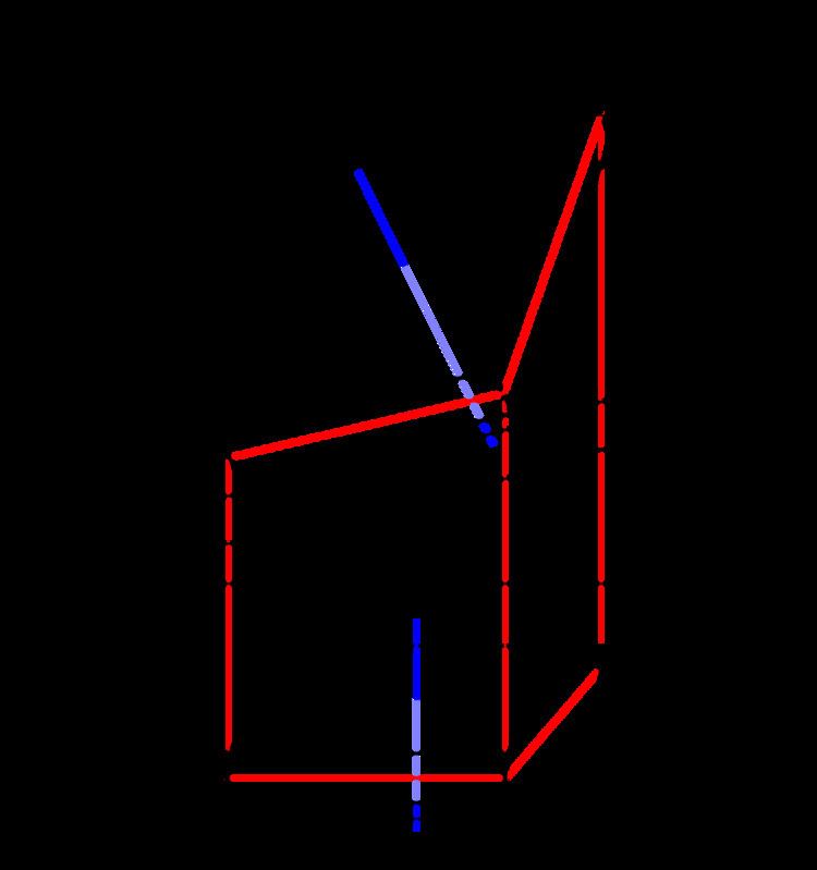
Let the position vector of a point in the undeformed plate be x . Then

x = x 1 e 1 + x 2 e 2 + x 3 e 3 ≡ x i e i .

The vectors e i form a Cartesian basis with origin on the mid-surface of the plate, x 1 and x 2 are the Cartesian coordinates on the mid-surface of the undeformed plate, and x 3 is the coordinate for the thickness direction.

Let the displacement of a point in the plate be u ( x ) . Then

u = u 1 e 1 + u 2 e 2 + u 3 e 3 ≡ u i e i

This displacement can be decomposed into a vector sum of the mid-surface displacement and an out-of-plane displacement w 0 in the x 3 direction. We can write the in-plane displacement of the mid-surface as

u 0 = u 1 0 e 1 + u 2 0 e 2 ≡ u α 0 e α

Note that the index α takes the values 1 and 2 but not 3.

Then the Kirchhoff hypothesis implies that

If φ α are the angles of rotation of the normal to the mid-surface, then in the Kirchhoff-Love theory

φ α = w , α 0

Note that we can think of the expression for u α as the first order Taylor series expansion of the displacement around the mid-surface.

Quasistatic Kirchhoff-Love plates

The original theory developed by Love was valid for infinitesimal strains and rotations. The theory was extended by von Kármán to situations where moderate rotations could be expected.

Strain-displacement relations

For the situation where the strains in the plate are infinitesimal and the rotations of the mid-surface normals are less than 10° the strain-displacement relations are

ε α β = 1 2 ( ∂ u α ∂ x β + ∂ u β ∂ x α ) ≡ 1 2 ( u α , β + u β , α ) ε α 3 = 1 2 ( ∂ u α ∂ x 3 + ∂ u 3 ∂ x α ) ≡ 1 2 ( u α , 3 + u 3 , α ) ε 33 = ∂ u 3 ∂ x 3 ≡ u 3 , 3

Using the kinematic assumptions we have

Therefore the only non-zero strains are in the in-plane directions.

Equilibrium equations

The equilibrium equations for the plate can be derived from the principle of virtual work. For a thin plate under a quasistatic transverse load q ( x ) these equations are

∂ N 11 ∂ x 1 + ∂ N 21 ∂ x 2 = 0 ∂ N 12 ∂ x 1 + ∂ N 22 ∂ x 2 = 0 ∂ 2 M 11 ∂ x 1 2 + 2 ∂ 2 M 12 ∂ x 1 ∂ x 2 + ∂ 2 M 22 ∂ x 2 2 = q

where the thickness of the plate is 2 h . In index notation,

where σ α β are the stresses.

Boundary conditions

The boundary conditions that are needed to solve the equilibrium equations of plate theory can be obtained from the boundary terms in the principle of virtual work. In the absence of external forces on the boundary, the boundary conditions are

n α N α β o r u β 0 n α M α β , β o r w 0 n β M α β o r w , α 0

Note that the quantity n α M α β , β is an effective shear force.

Constitutive relations

The stress-strain relations for a linear elastic Kirchhoff plate are given by

σ α β = C α β γ θ ε γ θ σ α 3 = C α 3 γ θ ε γ θ σ 33 = C 33 γ θ ε γ θ

Since σ α 3 and σ 33 do not appear in the equilibrium equations it is implicitly assumed that these quantities do not have any effect on the momentum balance and are neglected. The remaining stress-strain relations, in matrix form, can be written as

[ σ 11 σ 22 σ 12 ] = [ C 11 C 12 C 13 C 12 C 22 C 23 C 13 C 23 C 33 ] [ ε 11 ε 22 ε 12 ]

Then,

[ N 11 N 22 N 12 ] = ∫ − h h [ C 11 C 12 C 13 C 12 C 22 C 23 C 13 C 23 C 33 ] [ ε 11 ε 22 ε 12 ] d x 3 = { ∫ − h h [ C 11 C 12 C 13 C 12 C 22 C 23 C 13 C 23 C 33 ] d x 3 } [ u 1 , 1 0 u 2 , 2 0 1 2 ( u 1 , 2 0 + u 2 , 1 0 ) ]

and

[ M 11 M 22 M 12 ] = ∫ − h h x 3 [ C 11 C 12 C 13 C 12 C 22 C 23 C 13 C 23 C 33 ] [ ε 11 ε 22 ε 12 ] d x 3 = − { ∫ − h h x 3 2 [ C 11 C 12 C 13 C 12 C 22 C 23 C 13 C 23 C 33 ] d x 3 } [ w , 11 0 w , 22 0 w , 12 0 ]

The extensional stiffnesses are the quantities

A α β := ∫ − h h C α β d x 3

The bending stiffnesses (also called flexural rigidity) are the quantities

D α β := ∫ − h h x 3 2 C α β d x 3

The Kirchhoff-Love constitutive assumptions lead to zero shear forces. As a result, the equilibrium equations for the plate have to be used to determine the shear forces in thin Kirchhoff-Love plates. For isotropic plates, these equations lead to

Q α = − D ∂ ∂ x α ( ∇ 2 w 0 ) .

Alternatively, these shear forces can be expressed as

Q α = M , α

where

M := − D ∇ 2 w 0 .

Small strains and moderate rotations

If the rotations of the normals to the mid-surface are in the range of 10 ∘ to 15 ∘ , the strain-displacement relations can be approximated as

ε α β = 1 2 ( u α , β + u β , α + u 3 , α u 3 , β ) ε α 3 = 1 2 ( u α , 3 + u 3 , α ) ε 33 = u 3 , 3

Then the kinematic assumptions of Kirchhoff-Love theory lead to the classical plate theory with von Kármán strains

ε α β = 1 2 ( u α , β 0 + u β , α 0 + w , α 0 w , β 0 ) − x 3 w , α β 0 ε α 3 = − w , α 0 + w , α 0 = 0 ε 33 = 0

This theory is nonlinear because of the quadratic terms in the strain-displacement relations.

If the strain-displacement relations take the von Karman form, the equilibrium equations can be expressed as

N α β , α = 0 M α β , α β + [ N α β w , β 0 ] , α − q = 0

Isotropic quasistatic Kirchhoff-Love plates

For an isotropic and homogeneous plate, the stress-strain relations are

[ σ 11 σ 22 σ 12 ] = E 1 − ν 2 [ 1 ν 0 ν 1 0 0 0 1 − ν ] [ ε 11 ε 22 ε 12 ] .

The moments corresponding to these stresses are

[ M 11 M 22 M 12 ] = − 2 h 3 E 3 ( 1 − ν 2 ) [ 1 ν 0 ν 1 0 0 0 1 − ν ] [ w , 11 0 w , 22 0 w , 12 0 ]

In expanded form,

M 11 = − D ( ∂ 2 w 0 ∂ x 1 2 + ν ∂ 2 w 0 ∂ x 2 2 ) M 22 = − D ( ∂ 2 w 0 ∂ x 2 2 + ν ∂ 2 w 0 ∂ x 1 2 ) M 12 = − D ( 1 − ν ) ∂ 2 w 0 ∂ x 1 ∂ x 2

where D = 2 h 3 E / [ 3 ( 1 − ν 2 ) ] = H 3 E / [ 12 ( 1 − ν 2 ) ] for plates of thickness H = 2 h . Using the stress-strain relations for the plates, we can show that the stresses and moments are related by

σ 11 = 3 x 3 2 h 3 M 11 = 12 x 3 H 3 M 11 and σ 22 = 3 x 3 2 h 3 M 22 = 12 x 3 H 3 M 22 .

At the top of the plate where x 3 = h = H / 2 , the stresses are

σ 11 = 3 2 h 2 M 11 = 6 H 2 M 11 and σ 22 = 3 2 h 2 M 22 = 6 H 2 M 22 .

Pure bending

For an isotropic and homogeneous plate under pure bending, the governing equations reduce to

∂ 4 w 0 ∂ x 1 4 + 2 ∂ 4 w 0 ∂ x 1 2 ∂ x 2 2 + ∂ 4 w 0 ∂ x 2 4 = 0 .

Here we have assumed that the in-plane displacements do not vary with x 1 and x 2 . In index notation,

w , 1111 0 + 2 w , 1212 0 + w , 2222 0 = 0

and in direct notation

The bending moments are given by

[ M 11 M 22 M 12 ] = − 2 h 3 E 3 ( 1 − ν 2 ) [ 1 ν 0 ν 1 0 0 0 1 − ν ] [ w , 11 0 w , 22 0 w , 12 0 ]

Bending under transverse load

If a distributed transverse load − q ( x ) is applied to the plate, the governing equation is M α β , α β = − q . Following the procedure shown in the previous section we get

In rectangular Cartesian coordinates, the governing equation is

w , 1111 0 + 2 w , 1212 0 + w , 2222 0 = − q D

and in cylindrical coordinates it takes the form

1 r d d r [ r d d r { 1 r d d r ( r d w d r ) } ] = − q D .

Solutions of this equation for various geometries and boundary conditions can be found in the article on bending of plates.

Cylindrical bending

Under certain loading conditions a flat plate can be bent into the shape of the surface of a cylinder. This type of bending is called cylindrical bending and represents the special situation where u 1 = u 1 ( x 1 ) , u 2 = 0 , w = w ( x 1 ) . In that case

[ N 11 N 22 N 12 ] = 2 h E ( 1 − ν 2 ) [ 1 ν 0 ν 1 0 0 0 1 − ν ] [ u 1 , 1 0 0 0 ]

and

[ M 11 M 22 M 12 ] = − 2 h 3 E 3 ( 1 − ν 2 ) [ 1 ν 0 ν 1 0 0 0 1 − ν ] [ w , 11 0 0 0 ]

and the governing equations become

N 11 = A d u d x 1 ⟹ d 2 u d x 1 2 = 0 M 11 = − D d 2 w d x 1 2 ⟹ d 4 w d x 1 4 = q D

Dynamics of Kirchhoff-Love plates

The dynamic theory of thin plates determines the propagation of waves in the plates, and the study of standing waves and vibration modes.

Governing equations

The governing equations for the dynamics of a Kirchhoff-Love plate are

where, for a plate with density ρ = ρ ( x ) ,

J 1 := ∫ − h h ρ d x 3 = 2 ρ h ; J 3 := ∫ − h h x 3 2 ρ d x 3 = 2 3 ρ h 3

and

u ˙ i = ∂ u i ∂ t ; u ¨ i = ∂ 2 u i ∂ t 2 ; u i , α = ∂ u i ∂ x α ; u i , α β = ∂ 2 u i ∂ x α ∂ x β

Solutions of these equations for some special cases can be found in the article on vibrations of plates. The figures below show some vibrational modes of a circular plate.

Isotropic plates

The governing equations simplify considerably for isotropic and homogeneous plates for which the in-plane deformations can be neglected. In that case we are left with one equation of the following form (in rectangular Cartesian coordinates):

D ( ∂ 4 w ∂ x 4 + 2 ∂ 4 w ∂ x 2 ∂ y 2 + ∂ 4 w ∂ y 4 ) = − q ( x , y , t ) − 2 ρ h ∂ 2 w ∂ t 2 .

where D is the bending stiffness of the plate. For a uniform plate of thickness 2 h ,

D := 2 h 3 E 3 ( 1 − ν 2 ) .

In direct notation

D ∇ 2 ∇ 2 w = − q ( x , y , t ) − 2 ρ h w ¨ .

For free vibrations, the governing equation becomes

D ∇ 2 ∇ 2 w = − 2 ρ h w ¨ .

References

Kirchhoff–Love plate theory Wikipedia

(Text) CC BY-SA

Contents