
 | ||
In combinatorics (combinatorial mathematics), the inclusion–exclusion principle is a counting technique which generalizes the familiar method of obtaining the number of elements in the union of two finite sets; symbolically expressed as
Contents
- Statement
- Counting integers
- Counting derangements
- A special case
- A generalization
- In probability
- Special case
- Other forms
- Applications
- Counting intersections
- Graph coloring
- Bipartite graph perfect matchings
- Number of onto functions
- Permutations with forbidden positions
- Stirling numbers of the second kind
- Rook polynomials
- Eulers phi function
- Diluted inclusionexclusion principle
- Proof of main statement
- Algebraic proof
- References
where A and B are two finite sets and |S| indicates the cardinality of a set S (which may be considered as the number of elements of the set, if the set is finite). The formula expresses the fact that the sum of the sizes of the two sets may be too large since some elements may be counted twice. The double-counted elements are those in the intersection of the two sets and the count is corrected by subtracting the size of the intersection.
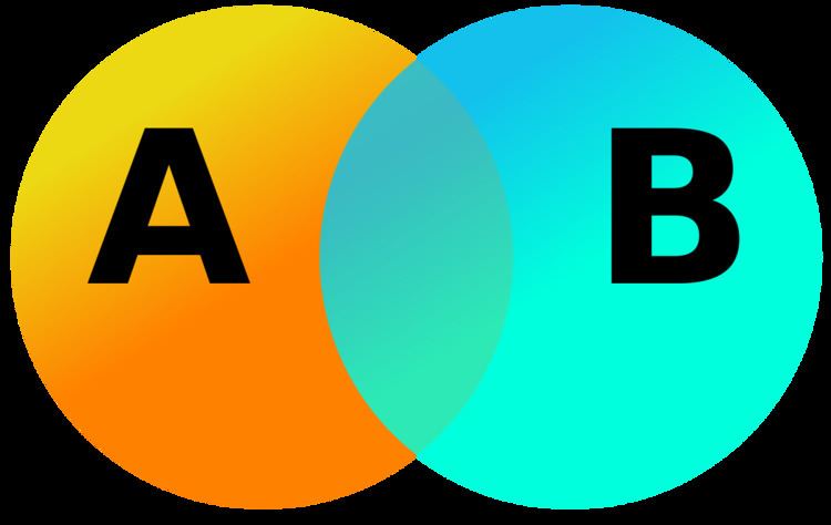
The principle is more clearly seen in the case of three sets, which for the sets A, B and C is given by
This formula can be verified by counting how many times each region in the Venn diagram figure is included in the right-hand side of the formula. In this case, when removing the contributions of over-counted elements, the number of elements in the mutual intersection of the three sets has been subtracted too often, so must be added back in to get the correct total.
Generalizing the results of these examples gives the principle of inclusion–exclusion. To find the cardinality of the union of n sets:
- Include the cardinalities of the sets.
- Exclude the cardinalities of the pairwise intersections.
- Include the cardinalities of the triple-wise intersections.
- Exclude the cardinalities of the quadruple-wise intersections.
- Include the cardinalities of the quintuple-wise intersections.
- Continue, until the cardinality of the n-tuple-wise intersection is included (if n is odd) or excluded (n even).
The name comes from the idea that the principle is based on over-generous inclusion, followed by compensating exclusion. This concept is attributed to Abraham de Moivre (1718); but it first appears in a paper of Daniel da Silva (1854), and later in a paper by J. J. Sylvester (1883). Sometimes the principle is referred to as the formula of Da Silva, or Sylvester due to these publications. The principle is an example of the sieve method extensively used in number theory and is sometimes referred to as the sieve formula, though Legendre already used a similar device in a sieve context in 1808.
As finite probabilities are computed as counts relative to the cardinality of the probability space, the formulas for the principle of inclusion–exclusion remain valid when the cardinalities of the sets are replaced by finite probabilities. More generally, both versions of the principle can be put under the common umbrella of measure theory.
In a very abstract setting, the principle of inclusion–exclusion can be expressed as the calculation of the inverse of a certain matrix. This inverse has a special structure, making the principle an extremely valuable technique in combinatorics and related areas of mathematics. As Gian-Carlo Rota put it:
"One of the most useful principles of enumeration in discrete probability and combinatorial theory is the celebrated principle of inclusion–exclusion. When skillfully applied, this principle has yielded the solution to many a combinatorial problem."
Statement
In its general form, the principle of inclusion–exclusion states that for finite sets A1, ..., An, one has the identity
This can be compactly written as
or
In words, to count the number of elements in a finite union of finite sets, first sum the cardinalities of the individual sets, then subtract the number of elements which appear in more than one set, then add back the number of elements which appear in more than two sets, then subtract the number of elements which appear in more than three sets, and so on. This process naturally ends since there can be no elements which appear in more than the number of sets in the union.
In applications it is common to see the principle expressed in its complementary form. That is, letting S be a finite universal set containing all of the Ai and letting
As another variant of the statement, let P1, P2, ..., Pn be a list of properties that elements of a set S may or may not have, then the principle of inclusion–exclusion provides a way to calculate the number of elements of S which have none of the properties. Just let Ai be the subset of elements of S which have the property Pi and use the principle in its complementary form. This variant is due to J. J. Sylvester.
Counting integers
As a simple example of the use of the principle of inclusion–exclusion, consider the question:
Let S = {1,...,100} and P1 the property that an integer is divisible by 2, P2 the property that an integer is divisible by 3 and P3 the property that an integer is divisible by 5. Letting Ai be the subset of S whose elements have property Pi we have by elementary counting: |A1| = 50, |A2| = 33, and |A3| = 20. There are 16 of these integers divisible by 6, 10 divisible by 10 and 6 divisible by 15. Finally, there are just 3 integers divisible by 30, so the number of integers not divisible by any of 2, 3 or 5 is given by:
Counting derangements
A more complex example is the following.
Suppose there is a deck of n cards numbered from 1 to n. Suppose a card numbered m is in the correct position if it is the mth card in the deck. How many ways, W, can the cards be shuffled with at least 1 card being in the correct position?
Begin by defining set Am, which is all of the orderings of cards with the mth card correct. Then the number of orders, W, with at least one card being in the correct position, m, is
Apply the principle of inclusion–exclusion,
Each value
Noting that
A permutation where no card is in the correct position is called a derangement. Taking n! to be the total number of permutations, the probability Q that a random shuffle produces a derangement is given by
a truncation to n + 1 terms of the Taylor expansion of e−1. Thus the probability of guessing an order for a shuffled deck of cards and being incorrect about every card is approximately 1/e or 37%.
A special case
The situation that appears in the derangement example above occurs often enough to merit special attention. Namely, when the size of the intersection sets appearing in the formulas for the principle of inclusion–exclusion depend only on the number of sets in the intersections and not on which sets appear. More formally, if the intersection
has the same cardinality, say αk = |AJ|, for every k-element subset J of {1, ..., n}, then
Or, in the complementary form, where the universal set S has cardinality α0,
A generalization
Given a family (repeats allowed) of subsets A1, A2, ..., An of a universal set S, the principle of inclusion–exclusion calculates the number of elements of S in none of these subsets. A generalization of this concept would calculate the number of elements of S which appear in exactly some fixed m of these sets.
Let N = [n] = {1,2,...,n}. If we define
If I is a fixed subset of the index set N, then the number of elements which belong to Ai for all i in I and for no other values is:
Define the sets
We seek the number of elements in none of the Bk which, by the principle of inclusion–exclusion (with
The correspondence K ↔ J = I ∪ K between subsets of N I and subsets of N containing I is a bijection and if J and K correspond under this map then BK = AJ, showing that the result is valid.
In probability
In probability, for events A1, ..., An in a probability space
for n = 3
and in general
which can be written in closed form as
where the last sum runs over all subsets I of the indices 1, ..., n which contain exactly k elements, and
denotes the intersection of all those Ai with index in I.
According to the Bonferroni inequalities, the sum of the first terms in the formula is alternately an upper bound and a lower bound for the LHS. This can be used in cases where the full formula is too cumbersome.
For a general measure space (S,Σ,μ) and measurable subsets A1, ..., An of finite measure, the above identities also hold when the probability measure
Special case
If, in the probabilistic version of the inclusion–exclusion principle, the probability of the intersection AI only depends on the cardinality of I, meaning that for every k in {1, ..., n} there is an ak such that
then the above formula simplifies to
due to the combinatorial interpretation of the binomial coefficient
An analogous simplification is possible in the case of a general measure space (S,Σ,μ) and measurable subsets A1, ..., An of finite measure.
Other forms
The principle is sometimes stated in the form that says that if
then
The combinatorial and the probabilistic version of the inclusion–exclusion principle are instances of (**).
If one sees a number
For a generalization of the full version of Möbius inversion formula, (**) must be generalized to multisets. For multisets instead of sets, (**) becomes
where
Notice that
Applications
The inclusion–exclusion principle is widely used and only a few of its applications can be mentioned here.
Counting derangements
A well-known application of the inclusion–exclusion principle is to the combinatorial problem of counting all derangements of a finite set. A derangement of a set A is a bijection from A into itself that has no fixed points. Via the inclusion–exclusion principle one can show that if the cardinality of A is n, then the number of derangements is [n! / e] where [x] denotes the nearest integer to x; a detailed proof is available here and also see the examples section above.
The first occurrence of the problem of counting the number of derangements is in an early book on games of chance: Essai d'analyse sur les jeux de hazard by P. R. de Montmort (1678 – 1719) and was known as either "Montmort's problem" or by the name he gave it, "problème des rencontres." The problem is also known as the hatcheck problem.
The number of derangements is also known as the subfactorial of n, written !n. It follows that if all bijections are assigned the same probability then the probability that a random bijection is a derangement quickly approaches 1/e as n grows.
Counting intersections
The principle of inclusion–exclusion, combined with De Morgan's law, can be used to count the cardinality of the intersection of sets as well. Let
thereby turning the problem of finding an intersection into the problem of finding a union.
Graph coloring
The inclusion exclusion principle forms the basis of algorithms for a number of NP-hard graph partitioning problems, such as graph coloring.
A well known application of the principle is the construction of the chromatic polynomial of a graph.
Bipartite graph perfect matchings
The number of perfect matchings of a bipartite graph can be calculated using the principle.
Number of onto functions
Given finite sets A and B, how many surjective functions (onto functions) are there from A to B? Without any loss of generality we may take A = {1,2,...,k} and B = {1,2,...,n}, since only the cardinalities of the sets matter. By using S as the set of all functions from A to B, and defining, for each i in B, the property Pi as "the function misses the element i in B" (i is not in the image of the function), the principle of inclusion–exclusion gives the number of onto functions between A and B as:
Permutations with forbidden positions
A permutation of the set S = {1,2,...,n} where each element of S is restricted to not being in certain positions (here the permutation is considered as an ordering of the elements of S) is called a permutation with forbidden positions. For example, with S = {1,2,3,4}, the permutations with the restriction that the element 1 can not be in positions 1 or 3, and the element 2 can not be in position 4 are: 2134, 2143, 3124, 4123, 2341, 2431, 3241, 3421, 4231 and 4321. By letting Ai be the set of positions that the element i is not allowed to be in, and the property Pi to be the property that a permutation puts element i into a position in Ai, the principle of inclusion–exclusion can be used to count the number of permutations which satisfy all the restrictions.
In the given example, there are 12 = 2(3!) permutations with property P1, 6 = 3! permutations with property P2 and no permutations have properties P3 or P4 as there are no restrictions for these two elements. The number of permutations satisfying the restrictions is thus:
The final 4 in this computation is the number of permutations having both properties P1 and P2. There are no other non-zero contributions to the formula.
Stirling numbers of the second kind
The Stirling numbers of the second kind, S(n,k) count the number of partitions of a set of n elements into k non-empty subsets (indistinguishable boxes). An explicit formula for them can be obtained by applying the principle of inclusion–exclusion to a very closely related problem, namely, counting the number of partitions of an n-set into k non-empty but distinguishable boxes (ordered non-empty subsets). Using the universal set consisting of all partitions of the n-set into k (possibly empty) distinguishable boxes, A1, A2, ..., Ak, and the properties Pi meaning that the partition has box Ai empty, the principle of inclusion–exclusion gives an answer for the related result. Dividing by k! to remove the artificial ordering gives the Stirling number of the second kind:
Rook polynomials
A rook polynomial is the generating function of the number of ways to place non-attacking rooks on a board B that looks like a subset of the squares of a checkerboard; that is, no two rooks may be in the same row or column. The board B is any subset of the squares of a rectangular board with n rows and m columns; we think of it as the squares in which one is allowed to put a rook. The coefficient, rk(B) of xk in the rook polynomial RB(x) is the number of ways k rooks, none of which attacks another, can be arranged in the squares of B. For any board B, there is a complementary board B' consisting of the squares of the rectangular board that are not in B. This complementary board also has a rook polynomial RB' (x) with coefficients rk(B').
It is sometimes convenient to be able to calculate the highest coefficient of a rook polynomial in terms of the coefficients of the rook polynomial of the complementary board. Without loss of generality we can assume that n ≤ m, so this coefficient is rn(B). The number of ways to place n non-attacking rooks on the complete n × m "checkerboard" (without regard as to whether the rooks are placed in the squares of the board B) is given by the falling factorial:
Letting Pi be the property that an assignment of n non-attacking rooks on the complete board has a rook in column i which is not in a square of the board B, then by the principle of inclusion–exclusion we have:
Euler's phi function
Euler's totient or phi function, φ(n) is an arithmetic function that counts the number of positive integers less than or equal to n that are relatively prime to n. That is, if n is a positive integer, then φ(n) is the number of integers k in the range 1 ≤ k ≤ n which have no common factor with n other than 1. The principle of inclusion–exclusion is used to obtain a formula for φ(n). Let S be the set {1,2,...,n} and define the property Pi to be that a number in S is divisible by the prime number pi, for 1 ≤ i ≤ r, where the prime factorization of
Then,
Diluted inclusion–exclusion principle
In many cases where the principle could give an exact formula (in particular, counting prime numbers using the sieve of Eratosthenes), the formula arising doesn't offer useful content because the number of terms in it is excessive. If each term individually can be estimated accurately, the accumulation of errors may imply that the inclusion–exclusion formula isn't directly applicable. In number theory, this difficulty was addressed by Viggo Brun. After a slow start, his ideas were taken up by others, and a large variety of sieve methods developed. These for example may try to find upper bounds for the "sieved" sets, rather than an exact formula.
Let A1, ..., An be arbitrary sets and p1, ..., pn real numbers in the closed unit interval [0,1]. Then, for every even number k in {0, ..., n}, the indicator functions satisfy the inequality:
Proof of main statement
Choose an element contained in the union of all sets and let
By the binomial theorem,
Using the fact that
and so, the chosen element is counted only once by the right-hand side of equation (1).
Algebraic proof
An algebraic proof can be obtained using indicator functions (characteristic functions of subsets of a set). The indicator function of a subset S of a set X is a function
defined as
If
Let A denote the union
for indicator functions, where
The following function is identically zero
because: if x is not in A, then all factors are 0 − 0 = 0; and otherwise, if x does belong to some Am, then the corresponding mth factor is 1 − 1 = 0. By expanding the product on the left-hand side, equation (∗) follows.
To prove the inclusion–exclusion principle for the cardinality of sets, sum the equation (∗) over all x in the union of A1, ..., An. To derive the version used in probability, take the expectation in (∗). In general, integrate the equation (∗) with respect to μ. Always use linearity in these derivations.