
 | ||
The hybrid difference scheme is a method used in the numerical solution for convection–diffusion problems. It was first introduces by Spalding (1970). It is a combination of central difference scheme and upwind difference scheme as it exploits the favorable properties of both of these schemes.
Contents
Introduction
Hybrid difference scheme is a method used in the numerical solution for convection-diffusion problems. These problems play important roles in computational fluid dynamics. It can be described by the general partial equation as follows:
Where,
For one-dimensional analysis of convection-diffusion problem in steady state and without the source the equation reduces to,
With boundary conditions,
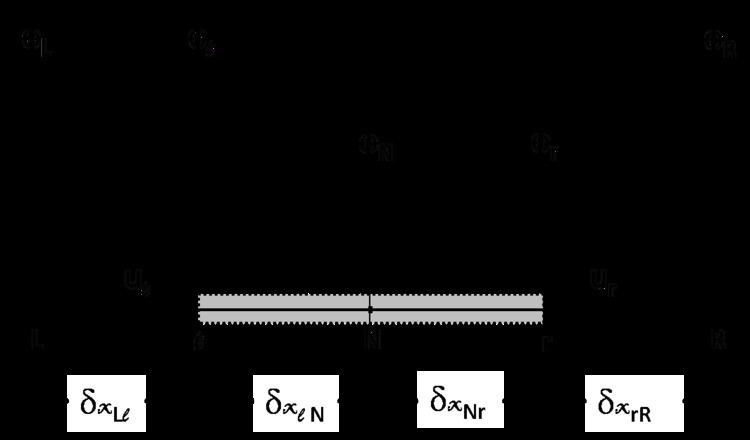
Grid generation
Integrating equation 2 over the control volume containing node N, and using the Gauss’ theorem i.e.,
Yields the following result,
Where, A is the cross-sectional area of the control volume. The equation must also satisfy the continuity equation, i.e.,
Now let us define variables F and D to represent the convection mass flux and diffusion conductance at cell faces,
Hence, equations (4) and (5) transform into the following equations:
Where, the lower case letters denote the values at the faces and the upper case letters denote that at the nodes. We also define a non-dimensional parameter Peclet number (Pe) as a measure of the relative strengths of convection and diffusion,
For a low Peclet number (|Pe|<2) the flow is characterized as dominated by diffusion. For large Peclet number the flow is dominated by convection.
Central and upwind difference scheme
In the above equations (7) and (8), we observe that the values require are at the faces, instead of the nodes. Hence approximations are required to fulfill this.
In the central difference scheme we replace the value at the face with the average of the values at the adjacent nodes,
By putting these values in equation (7) and rearranging we get the following result,
where,
In the Upwind scheme we replace the value at the face with the value at the adjacent upstream node. For example for the flow to the right (Pe>0)as shown in the diagram, we replace the values as follows;
And for Pe < 0, we put the values as shown in the figure 3,
By putting these values in equation (7) and rearranging we get the same equation as equation (11), with the following values of the coefficients:
Hybrid difference scheme
The hybrid difference scheme of Spalding (1970) is a combination of the central difference scheme and upwind difference scheme. It makes use of the central difference scheme, which is second order accurate, for small Peclet numbers (|Pe| < 2). For large Peclet numbers (|Pe| > 2) it uses the Upwind difference scheme, which first order accurate but takes into account the convection of the fluid.
As it can be seen in figure 4 that for Pe = 0, it is a linear distribution and for high Pe it takes the upstream value depending on the flow direction. For example the value at the left face, in different circumstances is,
Substituting these values in equation (7) we get the same equation (11) with the values of the coefficients as follows,
Advantages and disadvantages of the hybrid difference scheme
It exploits the favourable properties of the central difference and upwind scheme. It switches to upwind difference scheme when central difference scheme produces inaccurate results for high Peclet numbers. It produces physically realistic solution and has proved to be helpful in the prediction of practical flows.
The only disadvantage associated with hybrid difference scheme is that the accuracy in terms of Taylor series truncation error is only first order.