Central differencing scheme - Alchetron, the free social encyclopedia

In applied mathematics, the central differencing scheme is a finite difference method. The finite difference method optimizes the approximation for the differential operator in the central node of the considered patch and provides numerical solutions to differential equations. The central differencing scheme is one of the schemes used to solve the integrated convection-diffusion equation and to calculate the transported property Φ at the e and w faces. The advantages of this method are that it is easy to understand and to implement, at least for simple material relations, and that its convergence rate is faster than some other finite differencing methods, such as forward and backward differencing. The right hand side of the convection-diffusion equation which basically highlights the diffusion terms can be represented using central difference approximation. Thus, in order to simplify the solution and analysis, linear interpolation can be used logically to compute the cell face values for the left hand side of this equation which is nothing but the convective terms. Therefore cell face values of property for a uniform grid can be written as

Steady-state convection diffusion equation

The convection–diffusion equation is a collective representation of both diffusion and convection equations and describes or explains every physical phenomenon involving the two processes: convection and diffusion in transferring of particles, energy or other physical quantities inside a physical system. The convection-diffusion is as follows:

div ⁡ ( ρ u φ ) = div ⁡ ( Γ ∇ φ ) + S φ ;

here Г is diffusion coefficient and Φ is the property

Formulation of steady-state convection diffusion equation

Formal integration of steady-state convection–diffusion equation over a control volume gives

∫ A n ⋅ ( ρ u φ ) d A = ∫ A n ⋅ ( Γ ∇ φ ) d A + ∫ C V S φ d V → Equation 1.

This equation represents flux balance in a control volume. The left hand side gives the net convective flux and the right hand side contains the net diffusive flux and the generation or destruction of the property within the control volume.

In the absence of source term equation one becomes

d d x ( ρ u φ ) = d d x ( d φ d x ) → Equation 2.

Continuity equation:

d d x ( ρ u ) = 0 → Equation 3.

Assuming a control volume and integrating equation 2 over control volume gives:

( ρ u φ A ) e − ( ρ u φ A ) w = ( Γ A d φ / d x ) e − ( Γ A d φ / d x ) w → Integrated convection–diffusion equation

Integration of equation 3 yields:

( ρ u A ) e − ( ρ u A ) w = 0 → Integrated continuity equation

It is convenient to define two variables to represent the convective mass flux per unit area and diffusion conductance at cell faces which is as follows :

F = ρ u D = Γ / δ x

Assuming A e = A w , we can write integrated convection–diffusion equation as:

F e φ e − F w φ w = D e ( φ E − φ P ) − D w ( φ P − φ W )

And integrated continuity equation as:

F e − F w = 0

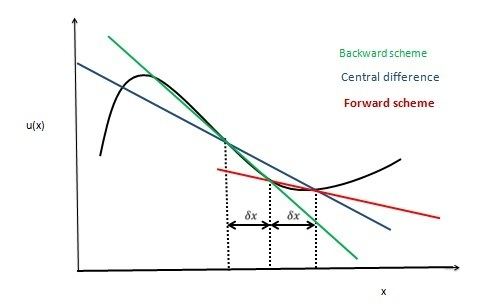
In central differencing scheme we try linear interpolation to compute cell face values for convection terms.

For a uniform grid we can write cell face values of property Φ as

φ e = ( φ E + φ P ) / 2 , φ w = ( φ P + φ W ) / 2

On substituting this into integrated convection – diffusion equation we obtain,

F e φ E + φ P 2 − F w φ W + φ P 2 = D e ( φ E − φ P ) − D w ( φ P − φ W )

And on rearranging,

[ ( D w + F w 2 ) + ( D e − F e 2 ) + ( F e − F w ) ] φ P = ( D w + F w 2 ) φ W + ( D e − F e 2 ) φ E

a P φ P = a W φ W + a E φ E

Conservativeness

Conservation is ensured in central differencing scheme since overall flux balance is obtained by summing the net flux through each control volume taking into account the boundary fluxes for the control volumes around nodes 1 and 4.

Boundary flux for control volume around node 1 and 4

[ Γ e 1 ( φ 2 − φ 1 ) δ x − q A ] + [ Γ e 2 ( φ 3 − φ 2 ) δ x − Γ w 2 ( φ 2 − φ 1 ) δ x ] + [ Γ e 3 ( φ 4 − φ 3 ) δ x − Γ w 3 ( φ 3 − φ 2 ) δ x ] + [ q B − Γ w 4 ( φ 4 − φ 3 ) δ x ] = q B − q A

because Γ e 1 = Γ w 2 , Γ e 2 = Γ w 3 , Γ e 3 = Γ w 4

Boundedness

Central differencing scheme satisfies first condition of Boundedness.

Since F e − F w = 0 from continuity equation, therefore; a P φ P = a W φ W + a E φ E

Another essential requirement for Boundedness is that all coefficients of the discretised equations should have the same sign (usually all positive). But this is only satisfied when (peclet number) F e / D e < 2 because for a unidirectional flow( F e > 0 , F w > 0 ) a E = ( D e − F e / 2 ) is always positive if D e > F e / 2

Transportiveness

It requires that transportiveness changes according to magnitude of peclet number i.e. when pe is zero φ is spread in all directions equally and as Pe increases (convection > diffusion) φ at a point largely depends on upstream value and less on downstream value. But central differencing scheme does not possess Transportiveness at higher pe since Φ at a point is average of neighbouring nodes for all Pe.

Accuracy

The Taylor series truncation error of the central differencing scheme is second order. Central differencing scheme will be accurate only if Pe < 2. Owing to this limitation central differencing is not a suitable discretisation practice for general purpose flow calculations.

Applications of central differencing scheme

Central difference type schemes are currently being applied on a regular basis in the solution of the Euler equations and Navier–Stokes equations.

The results using central differencing approximation have demonstrated noticeable improvements in accuracy in smooth regions.

Shock wave representation and boundary-layer definition can be improved on coarse meshes

Advantages

The central-difference schemes are simpler to program and require less computer time per time step, and work well with multigrid acceleration techniques.

The central difference schemes have a free parameter in conjunction with the fourth-difference dissipation.

This dissipation is needed to approach a steady state.

This scheme is more accurate than the first order upwind scheme if Peclet number is less than 2.

Disadvantages

The central differencing scheme is somewhat more dissipative.

This scheme leads to oscillations in the solution or divergence if the local Peclet number is larger than 2.

References

Central differencing scheme Wikipedia

(Text) CC BY-SA

Contents