Heterogeneous random walk in one dimension - Alchetron, the free social encyclopedia

In studies of dynamics, probability, physics, chemistry and related fields, a heterogeneous random walk in one dimension is a random walk in a one dimensional interval with jumping rules that depend on the location of the random walker in the interval.

For example: say that the time is discrete and also the interval. Namely, the random walker jumps every time step either left or right. A possible heterogeneous random walk draws in each time step a random number that determines the local jumping probabilities and then a random number that determines the actual jump direction. Specifically, say that the interval has 9 sites (labeled 1 through 9), and the sites (also termed states) are connected with each other linearly (where the edges sites are connected their adjacent sites and together). In each time step, the jump probabilities (from the actual site) are determined when flipping a coin; for head we set: probability jumping left =1/3, where for tail we set: probability jumping left = 0.55. Then, a random number is drawn from a uniform distribution: when the random number is smaller than probability jumping left, the jump is for the left, otherwise, the jump is for the right. Usually, in such a system, we are interested in the probability of staying in each of the various sites after t jumps, and in the limit of this probability when t is very large, t → ∞ .

Generally, the time in such processes can also vary in a continuous way, and the interval is also either discrete or continuous. Moreover, the interval is either finite or without bounds. In a discrete system, the connections are among adjacent states. The basic dynamics are either Markovian, semi-Markovian, or even not Markovian depending on the model. In discrete systems, heterogeneous random walks in 1d have jump probabilities that depend on the location in the system, and/or different jumping time (JT) probability density functions (PDFs) that depend on the location in the system.

General solutions for heterogeneous random walks in 1d obey equations (1)-(5), presented in what follows.

Random walks in applications

Random walks appear in the description of a wide variety of processes in biology, chemistry and physics. Random walks are used in describing chemical kinetics and polymer dynamics. In the evolving field of individual molecules, random walks supply the natural platform for describing the data. Namely, we see random walks when looking on individual molecules, individual channels, individual biomolecules, individual enzymes, quantum dots. Importantly, PDFs and special correlation functions can be easily calculated from single molecule measurements but not from ensemble measurements. This unique information can be used for discriminating between distinct random walk models that share some properties, and this demands a detailed theoretical analysis of random walk models. In this context, utilizing the information content in single molecule data is a matter of ongoing research.

Formulations of random walks

The actual random walk obeys a stochastic equation of motion. Yet, the probability density function (PDF) obeys a deterministic equation of motion. Formulation of PDFs of random walks can be done in terms of the discrete (in space) master equation and the generalized master equation or the continuum (in space and time) Fokker Planck equation and its generalizations. Continuous time random walks, renewal theory, and the path representation are also useful formulations of random walks. The network of relationships between the various descriptions provides a powerful tool in the analysis of random walks. Arbitrarily heterogeneous environments make the analysis difficult, especially in high dimensions.

Simple systems

Known important results in simple systems include:

In a symmetric Markovian random walk, the Green's function (also termed the PDF of the walker) for occupying state i is a Gaussian in the position and has a variance that scales like the time. This is correct for a system with discrete time and space, yet also in a system with continuous time and space. This results is for systems without bounds.

When there is a simple bias in the system (i.e. a constant force is applied on the system in a particular direction), the average distance of the random walker from its starting position is linear with time.

When trying reaching a distance L from the starting position in a finite interval of length L, the time τ for reaching this distance is exponential with the length L: τ = e L . Here, the diffusion is against a linear potential.

Heterogeneous systems

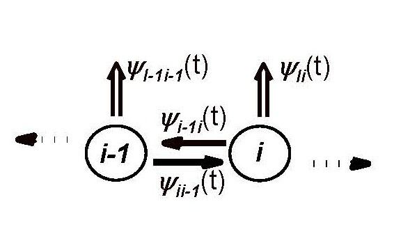
The solution for the Green's function G i j ( t ; L ) for a semi-Markovian random walk in an arbitrarily heterogeneous environment in 1D was recently given using the path representation. (The function G i j ( t ; L ) is the PDF for occupying state i at time t given that the process started at state j exactly at time 0.) A semi-Markovian random walk in 1D is defined as follows: a random walk whose dynamics are described by the (possibly) state- and direction-dependent JT-PDFs, ψ i j ( t ) , for transitions between states i and i ± 1, that generates stochastic trajectories of uncorrelated waiting times that are not-exponential distributed. ψ i j ( t ) obeys the normalization conditions (see fig. 1)

∑ j ∫ 0 ∞ ψ i j ( t ) = 1.

The dynamics can also include state- and direction-dependent irreversible trapping JT-PDFs, ψ i I ( t ) , with I=i+L. The environment is heterogeneous when ψ i j ( t ) depends on i. The above process is also a continuous time random walk and has an equivalent generalized master equation representation for the Green's function. G i j ( t ) .

Explicit expressions for heterogeneous random walks in 1D

In a completely heterogeneous semi-Markovian random walk in a discrete system of L (> 1) states, the Green's function was found in Laplace space (the Laplace transform of a function is defined with, f ¯ ( s ) = ∫ 0 ∞ e − s t f ( t ) d t ). Here, the system is defined through the jumping time (JT) PDFs: ψ i j ( t ) connecting state i with state j (the jump is from state i). The solution is based on the path representation of the Green's function, calculated when including all the path probability density functions of all lengths:

Here,

Ψ ¯ i ( s ) = ∑ j Ψ ¯ i j ( s )

and

Ψ ¯ i j ( s ) = 1 − ψ ¯ i j ( s ) s .

Also, in Eq. (1),

and

with

and

For L = 1, Φ ¯ ( s ; L ) = 1 . In this paper, the symbol [L/2], as appearing in the upper bound of the sum in eq. (5) is the floor operation (round towards zero). Finally, the factor Φ ( s , L ~ ) in eq. (1) has the same form as in Φ ¯ ( s ; L ) in eqs. (3)-(5), yet it is calculated on a lattice L ~ . Lattice L ~ is constructed from the original lattice by taking out from it the states i and j and the states between them, and then connecting the obtained two fragments. For cases in which a fragment is a single state, this fragment is excluded; namely, lattice L ~ is the longer fragment. When each fragment is a single state, Φ ¯ ( s ; L ~ ) = 1 .

Equations (1)-(5) hold for any 1D semi-Markovian random walk in a L-state chain, and form the most general solution in an explicit form for random walks in 1d.

Path representation of heterogeneous random walks

Clearly, G ¯ i j ( s ; L ) in Eqs. (1)-(5) solves the corresponding continuous time random walk problem and the equivalent generalized master equation. Equations (1)-(5) enable analyzing semi-Markovian random walks in 1D chains from a wide variety of aspects. Inversion to time domain gives the Green’s function, but also moments and correlation functions can be calculated from Eqs. (1)-(5), and then inverted into time domain (for relevant quantities). The closed-form G ¯ i j ( s ; L ) also manifests its utility when numerical inversion of the generalized master equation is unstable. Moreover, using G ¯ i j ( s ; L ) in simple analytical manipulations gives, (i) the first passage time PDF, (ii)–(iii) the Green’s functions for a random walk with a special WT-PDF for the first event and for a random walk in a circular L-state 1D chain, and (iv) joint PDFs in space and time with many arguments.

Still, the formalism used in this article is the path representation of the Green's function G i j ( t ) , and this supplies further information on the process. The path representation follows:

The expression for W i j ( t ; L ) in Eq. (6) follows,

W i j ( t ; L ) is the PDF of reaching state i exactly at time t when starting at state j exactly at time 0. This is the path PDF in time that is built from all paths with 2 n + γ i j transitions that connect states j with i. Two different path types contribute to w i j ( τ , 2 n + γ i j ; L ) : paths made of the same states appearing in different orders and different paths of the same length of 2 n + γ i j transitions. Path PDFs for translation invariant chains are mono-peaked. Path PDF for translation invariant chains mostly contribute to the Green's function in the vicinity of its peak, but this behavior is believed to characterize heterogeneous chains as well.

We also note that the following relation holds, W ¯ i j ( s ; L ) = W ¯ 1 L ( s ; L ) / W ¯ 1 L ~ ( s ; L ~ ) . Using this relation, we focus in what follows on solving w ¯ 1 L ( s ; L ) .

Path PDFs

Complementary information on the random walk with that supplied with the Green’s function is contained in path PDFs. This is evident, when constructing approximations for Green’s functions, in which path PDFs are the building blocks in the analysis. Also, analytical properties of the Green’s function are clarified only in path PDF analysis. Here, presented is the recursion relation for w i j ( τ , 2 n + γ i j ; L ) in the length n of path PDFs for any fixed value of L. The recursion relation is linear in path PDFs with the h ¯ ( s , i ; L ) s in Eq. (5) serving as the n independent coefficients, and is of order [L / 2]:

The recursion relation is used for explaining the universal formula for the coefficients in Eq. (1). The solution of the recursion relation is obtained by applying a z transform:

Setting z = 1 in Eq. (9) gives W ¯ 1 L ( s ; L ) . The Taylor expansion of Eq. (9) gives w ¯ 1 L ( s , 2 n + γ 1 L ; L ) . The result follows:

In Eq. (10) c ¯ k 0 ( s ; L ) is one for L = 2 , 3 , and otherwise,

where

The initial number a i , n s follow:

and,

References

Heterogeneous random walk in one dimension Wikipedia

(Text) CC BY-SA

Contents