Renewal theory

Introduction

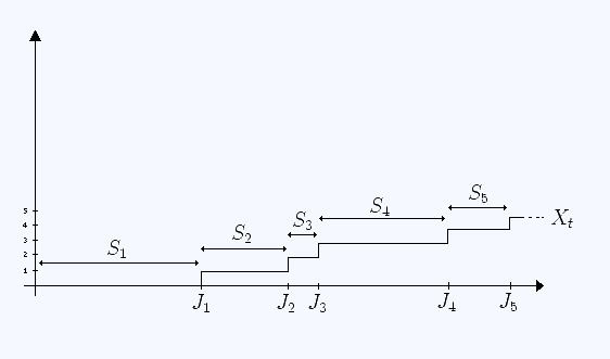
A renewal process is a generalization of the Poisson process. In essence, the Poisson process is a continuous-time Markov process on the positive integers (usually starting at zero) which has independent identically distributed holding times at each integer i (exponentially distributed) before advancing (with probability 1) to the next integer: i + 1 . In the same informal spirit, we may define a renewal process to be the same thing, except that the holding times take on a more general distribution. (Note however that the independence and identical distribution (IID) property of the holding times is retained).

Formal definition

Let S 1 , S 2 , S 3 , S 4 , S 5 , … be a sequence of positive independent identically distributed random variables such that

0 < E [ S i ] < ∞ .

We refer to the random variable S i as the " i -th" holding time.

E [ S i ] is the expectation of S i .

Define for each n > 0 :

J n = ∑ i = 1 n S i ,

each J n is referred to as the " n -th" jump time and the intervals

[ J n , J n + 1 ]

being called renewal intervals.

Then the random variable ( X t ) t ≥ 0 given by

X t = ∑ n = 1 ∞ I { J n ≤ t } = sup { n : J n ≤ t }

where I { J n ≤ t } is the indicator function

I { J n ≤ t } = { 1 , if  J n ≤ t 0 , otherwise

X t represents the number of jumps that have occurred by time t, and is called a renewal process.

Interpretation

If one considers events occurring at random times, one may choose to think of the holding times { S i : i ≥ 1 } as the random time elapsed between two subsequent events. For example, if the renewal process is modelling the breakdown of different machines, then the holding times represent the time between one machine breaking down before another one does.

Renewal-reward processes

Let W 1 , W 2 , … be a sequence of IID random variables (rewards) satisfying

E | W i | < ∞ .

Then the random variable

Y t = ∑ i = 1 X t W i

is called a renewal-reward process. Note that unlike the S i , each W i may take negative values as well as positive values.

The random variable Y t depends on two sequences: the holding times S 1 , S 2 , … and the rewards W 1 , W 2 , … These two sequences need not be independent. In particular, W i may be a function of S i .

Interpretation

In the context of the above interpretation of the holding times as the time between successive malfunctions of a machine, the "rewards" W 1 , W 2 , … (which in this case happen to be negative) may be viewed as the successive repair costs incurred as a result of the successive malfunctions.

An alternative analogy is that we have a magic goose which lays eggs at intervals (holding times) distributed as S i . Sometimes it lays golden eggs of random weight, and sometimes it lays toxic eggs (also of random weight) which require responsible (and costly) disposal. The "rewards" W i are the successive (random) financial losses/gains resulting from successive eggs (i = 1,2,3,...) and Y t records the total financial "reward" at time t.

Properties of renewal processes and renewal-reward processes

We define the renewal function as the expected value of the number of jumps observed up to some time t :

m ( t ) = E [ X t ] .

The elementary renewal theorem

The renewal function satisfies

lim t → ∞ 1 t m ( t ) = 1 / E [ S 1 ] .

Proof

Below, you find that the strong law of large numbers for renewal processes tell us that

lim t → ∞ X t t = 1 E [ S 1 ] .

To prove the elementary renewal theorem, it is sufficient to show that { X t t ; t ≥ 0 } is uniformly integrable.

To do this, consider some truncated renewal process where the holding times are defined by S n ¯ = a I { S n > a } where a is a point such that 0 < F ( a ) = p < 1 which exists for all non-deterministic renewal processes. This new renewal process X t ¯ is an upper bound on X t and its renewals can only occur on the lattice { n a ; n ∈ N } . Furthermore, the number of renewals at each time is geometric with parameter p . So we have

X t ¯ ≤ ∑ i = 1 [ a t ] G e o m e t r i c ( p ) E [ X t ¯ 2 ] ≤ C 1 t + C 2 t 2 P ( X t t > x ) ≤ E [ X t 2 ] t 2 x 2 ≤ E [ X t ¯ 2 ] t 2 x 2 ≤ C x 2 .

The elementary renewal theorem for renewal reward processes

We define the reward function:

g ( t ) = E [ Y t ] .

The reward function satisfies

lim t → ∞ 1 t g ( t ) = E [ W 1 ] E [ S 1 ] .

The renewal equation

The renewal function satisfies

m ( t ) = F S ( t ) + ∫ 0 t m ( t − s ) f S ( s ) d s

where F S is the cumulative distribution function of S 1 and f S is the corresponding probability density function.

Proof of the renewal equation

We may iterate the expectation about the first holding time: But by the Markov property So as required.

Asymptotic properties

( X t ) t ≥ 0 and ( Y t ) t ≥ 0 satisfy

lim t → ∞ 1 t X t = 1 E S 1 (strong law of large numbers for renewal processes) lim t → ∞ 1 t Y t = 1 E S 1 E W 1 (strong law of large numbers for renewal-reward processes)

almost surely.

Proof

First consider ( X t ) t ≥ 0 . By definition we have: for all t ≥ 0 and so for all t ≥ 0. Now since 0 < E S i < ∞ we have: as t → ∞ almost surely (with probability 1). Hence: almost surely (using the strong law of large numbers); similarly: almost surely. Thus (since t / X t is sandwiched between the two terms) almost surely. Next consider ( Y t ) t ≥ 0 . We have almost surely (using the first result and using the law of large numbers on Y t ).

The inspection paradox

A curious feature of renewal processes is that if we wait some predetermined time t and then observe how large the renewal interval containing t is, we should expect it to be typically larger than a renewal interval of average size.

Mathematically the inspection paradox states: for any t > 0 the renewal interval containing t is stochastically larger than the first renewal interval. That is, for all x > 0 and for all t > 0:

P ( S X t + 1 > x ) ≥ P ( S 1 > x ) = 1 − F S ( x )

where F_S is the cumulative distribution function of the IID holding times S_i.

Proof of the inspection paradox

Observe that the last jump-time before t is J X t ; and that the renewal interval containing t is S X t + 1 . Then

P ( S X t + 1 > x ) = ∫ 0 ∞ P ( S X t + 1 > x ∣ J X t = s ) f S ( s ) d s = ∫ 0 ∞ P ( S X t + 1 > x | S X t + 1 > t − s ) f S ( s ) d s = ∫ 0 ∞ P ( S X t + 1 > x , S X t + 1 > t − s ) P ( S X t + 1 > t − s ) f S ( s ) d s = ∫ 0 ∞ 1 − F ( max { x , t − s } ) 1 − F ( t − s ) f S ( s ) d s = ∫ 0 ∞ min { 1 − F ( x ) 1 − F ( t − s ) , 1 − F ( t − s ) 1 − F ( t − s ) } f S ( s ) d s = ∫ 0 ∞ min { 1 − F ( x ) 1 − F ( t − s ) , 1 } f S ( s ) d s ≥ 1 − F ( x ) = P ( S 1 > x )

as required.

Superposition

The superposition of independent renewal processes is not generally a renewal process, but it can be described within a larger class of processes called the Markov-renewal processes. However, the cumulative distribution function of the first inter-event time in the superposition process is given by

where R_k(t) and α_k > 0 are the CDF of the inter-event times and the arrival rate of process k.

Example 1: use of the strong law of large numbers

Eric the entrepreneur has n machines, each having an operational lifetime uniformly distributed between zero and two years. Eric may let each machine run until it fails with replacement cost €2600; alternatively he may replace a machine at any time while it is still functional at a cost of €200.

What is his optimal replacement policy?

Solution

The lifetime of the n machines can be modeled as n independent concurrent renewal-reward processes, so it is sufficient to consider the case n=1. Denote this process by ( Y t ) t ≥ 0 . The successive lifetimes S of the replacement machines are independent and identically distributed, so the optimal policy is the same for all replacement machines in the process.

If Eric decides at the start of a machine's life to replace it at time 0 < t < 2 but the machine happens to fail before that time then the lifetime S of the machine is uniformly distributed on [0, t] and thus has expectation 0.5t. So the overall expected lifetime of the machine is:

E S = E [ S ∣ fails before  t ] ⋅ P [ fails before  t ] + E [ S ∣ does not fail before  t ] ⋅ P [ does not fail before  t ] = t 2 ( 0.5 t ) + 2 − t 2 ( t )

and the expected cost W per machine is:

E W = E ( W ∣ fails before  t ) ⋅ P ( fails before  t ) + E ( W ∣ does not fail before  t ) ⋅ P ( does not fail before  t ) = t 2 ( 2600 ) + 2 − t 2 ( 200 ) = 1200 t + 200.

So by the strong law of large numbers, his long-term average cost per unit time is:

1 t Y t ≃ E W E S = 4 ( 1200 t + 200 ) t 2 + 4 t − 2 t 2

then differentiating with respect to t:

∂ ∂ t 4 ( 1200 t + 200 ) t 2 + 4 t − 2 t 2 = 4 ( 4 t − t 2 ) ( 1200 ) − ( 4 − 2 t ) ( 1200 t + 200 ) ( t 2 + 4 t − 2 t 2 ) 2 ,

this implies that the turning points satisfy:

0 = ( 4 t − t 2 ) ( 1200 ) − ( 4 − 2 t ) ( 1200 t + 200 ) = 4800 t − 1200 t 2 − 4800 t − 800 + 2400 t 2 + 400 t = − 800 + 400 t + 1200 t 2 ,

and thus

0 = 3 t 2 + t − 2 = ( 3 t − 2 ) ( t + 1 ) .

We take the only solution t in [0, 2]: t = 2/3. This is indeed a minimum (and not a maximum) since the cost per unit time tends to infinity as t tends to zero, meaning that the cost is decreasing as t increases, until the point 2/3 where it starts to increase.