Hermite distribution

Updated on Oct 23, 2023

Edit

Comment

Parameters a1 ≥ 0, a2 ≥ 0		Support x ∈ { 0, 1, 2, ... }

Notation H e r m ( a 1 , a 2 ) {\displaystyle \mathrm {Herm} (a_{1},a_{2})\,} pmf x ↦ e − ( a 1 + a 2 ) ∑ j = 0 ⌊ x / 2 ⌋ a 1 n − 2 j a 2 j ( n − 2 j ) ! j ! {\displaystyle x\mapsto e^{-(a_{1}+a_{2})}\sum _{j=0}^{\lfloor x/2\rfloor }{\frac {a_{1}^{n-2j}a_{2}^{j}}{(n-2j)!j!}}} CDF x ↦ e − a 1 + a 2 ∑ i = 0 ⌊ x ⌋ ∑ j = 0 [ i / 2 ] a 1 i − 2 j a 2 j ( i − 2 j ) ! j ! {\displaystyle x\mapsto e^{-a_{1}+a_{2}}\sum _{i=0}^{\lfloor x\rfloor }\sum _{j=0}^{[i/2]}{\frac {a_{1}^{i-2j}a_{2}^{j}}{(i-2j)!j!}}} Mean a 1 + 2 a 2 {\displaystyle a_{1}+2a_{2}}

In probability theory and statistics, the Hermite distribution, named after Charles Hermite, is a discrete probability distribution used to model count data with more than one parameter. This distribution is flexible in terms of its ability to allow a moderate over-dispersion in the data. The Hermite distribution is a special case of the Poisson binomial distribution, when n = 2.

The authors Kemp and Kemp have called it "Hermite distribution" from the fact its probability function and the moment generating function can be expressed in terms of the coefficients of (modified) Hermite polynomials.

History

The distribution first appeared in the paper Applications of Mathematics to Medical Problems, by Anderson Gray McKendrick in 1926. In this work the author explains several mathematical methods that can be applied to medical research. In one of this methods he considered the bivariate Poisson distribution and showed that the distribution of the sum of two correlated Poisson variables follow a distribution that later would be known as Hermite distribution.

As a practical application, McKendrick considered the distribution of counts of bacteria in leucocytes. Using the method of moments he fitted the data with the Hermite distribution and found the model more satisfactory than fitting it with a Poisson distribution.

The distribution was formally introduced and published by C. D. Kemp and Adrienne W.Kemp in 1965 in their work Some Properties of ‘Hermite’ Distribution. The work is focused on the properties of this distribution for instance a necessary condition on the parameters and their maximum likelihood estimators (MLE), the analysis of the probability generating function (PGF) and how it can be expressed in terms of the coefficients of (modified) Hermite polynomials. An example they have used in this publication is the distribution of counts of bacteria in leucocytes that used McKendrick but Kemp and Kemp estimate the model using the maximum likelihood method.

Hermite distribution is a special case of discrete compound Poisson distribution with only two parameters.

The same authors published in 1966 the paper An alternative Derivation of the Hermite Distribution. In this work established that the Hermite distribution can be obtained formally by combining a Poisson distribution with a normal distribution.

In 1971, Y. C. Patel did a comparative study of various estimation procedures for the Hermite distribution in his doctoral thesis. It included maximum likelihood, moment estimators, mean and zero frequency estimators and the method of even points.

In 1974, Gupta and Jain did a research on a generalized form of Hermite distribution.

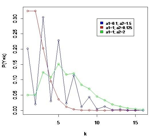
Probability mass function

Let X₁ and X₂ be two independent Poisson variables with parameters a₁ and a₂. The probability distribution of the random variable Y = X₁ + 2X₂ is the Hermite distribution with parameters a₁ and a₂ and probability mass function is given by

p n = P ( Y = n ) = e − a 1 + a 2 ∑ j = 0 [ n / 2 ] a 1 n − 2 j a 2 j ( n − 2 j ) ! j !

where

n = 0, 1, 2, ...

a₁, a₂ ≥ 0.

(n − 2j)! and j! are the factorials of (n − 2j) and j, respectively.

[n/2] is the integer part of [n/2].

The probability generating function of the probability mass is,

G Y ( s ) = ∑ n = 0 ∞ p n s n = exp ⁡ ( a 1 ( s − 1 ) + a 2 ( s 2 − 1 ) )

Notation

When a random variable Y = X₁ + 2X₂ is distributed by an Hermite distribution, where X₁ and X₂ are two independent Poisson variables with parameters a₁ and a₂, we write

Y ∼ H e r m ( a 1 , a 2 )

Moment and cumulant generating functions

The moment generating function of a random variable X is defined as the expected value of e^t, as a function of the real parameter t. For an Hermite distribution with parameters X₁ and X₂, the moment generating function exists and is equal to

M ( t ) = G ( e t ) = exp ⁡ ( a 1 ( e t − 1 ) + a 2 ( e 2 t − 1 ) )

The cumulant generating function is the logarithm of the moment generating function and is equal to

K ( t ) = log ⁡ ( M ( t ) ) = a 1 ( e t − 1 ) + a 2 ( e 2 t − 1 )

If we consider the coefficient of (it)^rr! in the expansion of K(t) we obtain the r-cumulant

k n = a 1 + 2 n a 2

Hence the mean and the succeeding three moments about it are

Skewness

The skewness is the third moment centered around the mean divided by the 3/2 power of the standard deviation, and for the hermite distribution is,

γ 1 = μ 3 μ 2 3 / 2 = ( a 1 + 8 a 2 ) ( a 1 + 4 a 2 ) 3 / 2

Always γ 1 > 0 , so the mass of the distribution is concentrated on the left.

Kurtosis

The kurtosis is the fourth moment centered around the mean, divided by the square of the variance, and for the Hermite distribution is,

β 2 = μ 4 μ 2 2 = a 1 + 16 a 2 + 3 ( a 1 + 4 a 2 ) 2 ( a 1 + 4 a 2 ) 2 = a 1 + 16 a 2 ( a 1 + 4 a 2 ) 2 + 3

The excess kurtosis is just a correction to make the kurtosis of the normal distribution equal to zero, and it is the following,

γ 2 = μ 4 μ 2 2 − 3 = a 1 + 16 a 2 ( a 1 + 4 a 2 ) 2

Always β 2 > 3 , or γ 2 > 0 the distribution has a high acute peak around the mean and fatter tails.

Characteristic function

In a discrete distribution the characteristic function of any real-valued random variable is defined as the expected value of e i t X , where i is the imaginary unit and t ∈ R

ϕ ( t ) = E [ e i t X ] = ∑ j = 0 ∞ e i j t P [ X = j ]

This function is related to the moment-generating function via ϕ x ( t ) = M X ( i t ) . Hence for this distribution the characteristic function is,

ϕ x ( t ) = exp ⁡ ( a 1 ( e i t − 1 ) + a 2 ( e 2 i t − 1 ) )

Cumulative distribution function

The cumulative distribution function is,

F ( x ; a 1 , a 2 ) = P ( X ≤ x ) = exp ⁡ ( − ( a 1 + a 2 ) ) ∑ i = 0 ⌊ x ⌋ ∑ j = 0 [ i / 2 ] a 1 i − 2 j a 2 j ( i − 2 j ) ! j !

Other properties

This distribution can have any number of modes. As an example, the fitted distribution for McKendrick’s data has an estimated parameters of a 1 ^ = 0.0135 , a 2 ^ = 0.0932 . Therefore, the first five estimated probabilities are 0.899, 0.012, 0.084, 0.001, 0.004.

This distribution is closed under addition or closed under convolutions. As the Poisson distribution, the Hermite distribution has this property. Given 2 random Hermite variables X 1 ∼ H e r m ( a 1 , a 2 ) and X 2 ∼ H e r m ( b 1 , b 2 ) , then Y = X₁ + X₂ follows an Hermite distribution, Y ∼ H e r m ( a 1 + b 1 , a 2 + b 2 ) .

This distribution allows a moderate overdispersion, so it can be used when data has this property. A random variable has overdispersion, or it is overdispersed with respect the Poisson distribution, when its variance is greater than its expected value. The Hermite distribution allows a moderate overdispersion because the coefficient of dispersion is always between 1 and 2,

Method of moments

The mean and the variance of the Hermite distribution are μ = a 1 + 2 a 2 and σ 2 = a 1 + 4 a 2 , respectively. So we have these two equation,

{ x ¯ = a 1 + 2 a 2 σ 2 = a 1 + 4 a 2

Solving these two equation we get the moment estimators a 1 ^ and a 2 ^ of a₁ and a₂.

a 1 ^ = 2 x ¯ − σ 2 a 2 ^ = σ 2 − x ^ 2

Since a₁ and a₂ both are positive, the estimator a 1 ^ and a 2 ^ are admissible (≥ 0) only if, x ¯ < σ 2 < 2 x ¯ .

Maximum likelihood

Given a sample X₁, ..., X_m are independent random variables each having an Hermite distribution we wish to estimate the value of the parameters a 1 ^ and a 2 ^ . We know that the mean and the variance of the distribution are μ = a 1 + 2 a 2 and σ 2 = a 1 + 4 a 2 , respectively. Using these two equation,

{ a 1 = μ ( 2 − d ) a 2 = μ ( d − 1 ) 2

We can parameterize the probability function by μ and d

P ( X = x ) = exp ⁡ ( − ( μ ( 2 − d ) + μ ( d − 1 ) 2 ) ) ∑ j = 0 [ x / 2 ] ( μ ( 2 − d ) ) x − 2 j ( μ ( d − 1 ) 2 ) j ( x − 2 j ) ! j !

Hence the log-likelihood function is,

L ( x 1 , … , x m ; μ , d ) = log ⁡ ( L ( x 1 , … , x m ; μ , d ) ) = m μ ( − 1 + d − 1 2 ) + log ⁡ ( μ ( 2 − d ) ) ∑ i = 1 m x i + ∑ i = 1 m log ⁡ ( q i ( θ ) )

where

q i ( θ ) = ∑ j = 0 [ x i / 2 ] θ j ( x i − 2 j ) ! j !

θ = d − 1 2 μ ( 2 − d ) 2

From the log-likelihood function, the likelihood equations are,

∂ l ∂ μ = m ( − 1 + d − 1 2 ) + 1 μ ∑ i = 1 m x i − d − 1 2 μ 2 ( 2 − d ) 2 ∑ i = 1 m q i ′ ( θ ) q i ( θ ) ∂ l ∂ d = m μ 2 − ∑ i = 1 m x i 2 − d − d 2 μ ( 2 − d ) 3 ∑ i = 1 m ∑ i = 1 m q i ′ ( θ ) q i ( θ )

Straightforward calculations show that,

μ = x ¯

And d can be found by solving,

where θ ~ = d − 1 2 x ¯ ( 2 − d ) 2

It can be shown that the log-likelihood function is strictly concave in the domain of the parameters. Consequently, the MLE is unique.

The likelihood equation does not always have a solution like as it shows the following proposition,

Proposition: Let X₁, ..., X_m come from a generalized Hermite distribution with fixed n. Then the MLEs of the parameters are μ ^ and d ~ if only if m ( 2 ) / x ¯ 2 > 1 , where m ( 2 ) = ∑ i = 1 n x i ( x i − 1 ) / n indicates the empirical factorial momement of order 2.

Remark 1: The condition m ( 2 ) / x ¯ 2 > 1 is equivalent to d ~ > 1 where d ~ = σ 2 / x ¯ is the empirical dispersion index

Remark 2: If the condition is not satisfied, then the MLEs of the parameters are μ ^ = x ¯ and d ~ = 1 , that is, the data are fitted using the Poisson distribution.

Zero frequency and the mean estimators

A usual choice for discrete distributions is the zero relative frequency of the data set which is equated to the probability of zero under the assumed distribution. Observing that f 0 = exp ⁡ ( − ( a 1 + a 2 ) ) and μ = a 1 + 2 a 2 . Following the example of Y. C. Patel (1976) the resulting system of equations,

{ x ¯ = a 1 + 2 a 2 f 0 = exp ⁡ ( − ( a 1 + a 2 ) )

We obtain the zero frequency and the mean estimator a₁ of a 1 ^ and a₂ of a 2 ^ ,

a 1 ^ = − ( x ¯ + 2 log ⁡ ( f 0 ) ) a 2 ^ = x ¯ + log ⁡ ( f 0 )

where f 0 = n 0 n , is the zero relative frequency, n > 0

It can be seen that for distributions with a high probability at 0, the efficiency is high.

For admissible values of a 1 ^ and a 2 ^ , we must have

Testing Poisson assumption

When Hermite distribution is used to model a data sample is important to check if the Poisson distribution is enough to fit the data. Following the parametrized probability mass function used to calculate the maximum likelihood estimator, is important to corroborate the following hypothesis,

{ H 0 : d = 1 H 1 : d > 1

Likelihood-ratio test

The likelihood-ratio test statistic for hermite distribution is,

W = 2 ( L ( X ; μ ^ , d ^ ) − L ( X ; μ ^ , 1 ) )

Where L ( ) is the log-likelihood function. As d = 1 belongs to the boundary of the domain of parameters, under the null hypothesis, W does not have an asymptotic χ 1 2 distribution as expected. It can be established that the asymptotic distribution of W is a 50:50 mixture of the constant 0 and the χ 1 2 . The α upper-tail percentage points for this mixture are the same as the 2α upper-tail percentage points for a χ 1 2 ; for instance, for α = 0.01, 0.05, and 0.10 they are 5.41189, 2.70554 and 1.64237.

The "score" or Lagrange multiplier test

The score statistic is,

S 2 = 2 m [ m ( 2 ) − x ¯ 2 2 x ¯ ] 2 = m ( d ~ − 1 ) 2 2

where m is the number of observations.

The asymptotic distribution of the score test statistic under the null hypothesis is a χ 1 2 distribution. It may be convenient to use a signed version of the score test, that is, sgn ⁡ ( m ( 2 ) − x ¯ 2 ) S , following asymptotically a standard normal.

References

Hermite distribution Wikipedia

(Text) CC BY-SA

Contents