Hamiltonian optics

Hamilton's principle

In physics, Hamilton's principle states that the evolution of a system ( q 1 ( σ ) , ⋯ , q N ( σ ) ) described by N generalized coordinates between two specified states at two specified parameters σ_A and σ_B is a stationary point (a point where the variation is zero), of the action functional, or

where q ˙ k = d q k / d σ . Condition δ S = 0   is valid if and only if the Euler-Lagrange equations are satisfied

with k = 1 , ⋯ , N .

The momentum is defined as

and the Euler-Lagrange equations can then be rewritten as

where p ˙ k = d p k / d σ .

A different approach to solving this problem consists in defining a Hamiltonian (taking a Legendre transform of the Lagrangian) as

for which a new set of differential equations can be derived by looking at how the total differential of the Lagrangian depends on parameter σ, positions q i and their derivatives q ˙ i relative to σ. This derivation is the same as in Hamiltonian mechanics, only with time t now replaced by a general parameter σ. Those differential equations are the Hamilton's equations

with k = 1 , ⋯ , N . Hamilton's equations are first-order differential equations, while Euler-Lagrange's equations are second-order.

Lagrangian and Hamiltonian optics

The general results presented above for Hamilton's principle can be applied to optics. In 3D euclidean space the generalized coordinates are now the coordinates of euclidean space.

Fermat's principle

Fermat's principle states that the optical length of the path followed by light between two fixed points, A and B, is a stationary point. It may be a maximum, a minimum, constant or an inflection point. In general, as light travels, it moves in a medium of variable refractive index which is a scalar field of position in space, that is, n = n ( x 1 , x 2 , x 3 )   in 3D euclidean space. Assuming now that light travels along the x₃ axis, the path of a light ray may be parametrized as s = ( x 1 ( x 3 ) , x 2 ( x 3 ) , x 3 )   starting at a point A = ( x 1 ( x 3 A ) , x 2 ( x 3 A ) , x 3 A )   and ending at a point B = ( x 1 ( x 3 B ) , x 2 ( x 3 B ) , x 3 B )   . In this case, when compared to Hamilton's principle above, coordinates x 1   and x 2   take the role of the generalized coordinates q k   while x 3   takes the role of parameter σ   , that is, parameter σ =x₃ and N=2.

In the context of calculus of variations this can be written as

where ds is an infinitesimal displacement along the ray given by d s = d x 1 2 + d x 2 2 + d x 3 2 and

is the optical Lagrangian and x ˙ k = d x k / d x 3 .

The optical path length (OPL) is defined as

where n is the local refractive index as a function of position along the path between points A and B.

The Euler-Lagrange equations

The general results presented above for Hamilton's principle can be applied to optics using the Lagrangian defined in Fermat's principle. The Euler-Lagrange equations with parameter σ =x₃ and N=2 applied to Fermat's principle result in

with k=1,2 and where L is the optical Lagrangian and x ˙ k = d x k / d x 3 .

Optical momentum

The optical momentum is defined as

and from the definition of the optical Lagrangian L = n 1 + x ˙ 1 2 + x ˙ 2 2 this expression can be rewritten as

or in vector form

where e ^ is a unit vector and angles α₁, α₂ and α₃ are the angles p makes to axis x₁, x₂ and x₃ respectively, as shown in figure "optical momentum". Therefore the optical momentum is a vector of norm

where n is the refractive index at which p is calculated. Vector p points in the direction of propagation of light. If light is propagating in a gradient index optic the path of the light ray is curved and vector p is tangent to the light ray.

The expression for the optical path length can also be written as a function of the optical momentum. Having in consideration that x ˙ 3 = d x 3 / d x 3 = 1 the expression for the optical Lagrangian can be rewritten as

and the expression for the optical path length is

Hamilton's equations

Similarly to what happens in Hamiltonian mechanics, also in optics the Hamiltonian is defined by the expression given above for N=2 corresponding to functions x 1 ( x 3 ) and x 2 ( x 3 ) to be determined

Comparing this expression with L = x ˙ 1 p 1 + x ˙ 2 p 2 + p 3 for the Lagrangian results in

And the corresponding Hamilton's equations with parameter σ =x₃ and k=1,2 applied to optics are

with x ˙ k = d x k / d x 3 and p ˙ k = d p k / d x 3 .

Applications

It is assumed that light travels along the x₃ axis, in Hamilton's principle above, coordinates x 1   and x 2   take the role of the generalized coordinates q k   while x 3   takes the role of parameter σ   , that is, parameter σ =x₃ and N=2.

Refraction and reflection

If plane x₁x₂ separates two media of refractive index n_A below and n_B above it, the refractive index is given by a step function

and from Hamilton's equations

and therefore p ˙ k = 0 or p k = Constant   for k=1,2.

An incoming light ray has momentum p_A before refraction (below plane x₁x₂) and momentum p_B after refraction (above plane x₁x₂). The light ray makes an angle θ_A with axis x₃ (the normal to the refractive surface) before refraction and an angle θ_B with axis x₃ after refraction. Since the p₁ and p₂ components of the momentum are constant, only p₃ changes from p_3A to p_3B.

Figure "refraction" shows the geometry of this refraction from which d = ∥ p A ∥ sin ⁡ θ A = ∥ p B ∥ sin ⁡ θ B . Since ∥ p A ∥ = n A and ∥ p B ∥ = n B , this last expression can be written as

which is Snell's law of refraction.

In figure "refraction", the normal to the refractive surface points in the direction of axis x₃, and also of vector v = p A − p B . A unit normal n = v / ∥ v ∥ to the refractive surface can then be obtained from the momenta of the incoming and outgoing rays by

where i and r are a unit vectors in the directions of the incident and refracted rays. Also, the outgoing ray (in the direction of p B ) is contained in the plane defined by the incoming ray (in the direction of p A ) and the normal n   to the surface.

A similar argument can be used for reflection in deriving the law of specular reflection, only now with n_A=n_B, resulting in θ_A=θ_B. Also, if i and r are unit vectors in the directions of the incident and refracted ray respectively, the corresponding normal to the surface is given by the same expression as for refraction, only with n_A=n_B

In vector form, if i is a unit vector pointing in the direction of the incident ray and n is the unit normal to the surface, the direction r of the refracted ray is given by:

with

If i·n<0 then -n should be used in the calculations. When Δ < 0 , light suffers total internal reflection and the expression for the reflected ray is that of reflection:

Rays and wavefronts

From the definition of optical path length S = ∫ L d x 3

with k=1,2 where the Euler-Lagrange equations ∂ L / ∂ x k = d p k / d x 3 with k=1,2 were used. Also, from the last of Hamilton's equations ∂ H / ∂ x 3 = − ∂ L / ∂ x 3 and from H = − p 3   above

combining the equations for the components of momentum p results in

Since p is a vector tangent to the light rays, surfaces S=Constant must be perpendicular to those light rays. These surfaces are called wavefronts. Figure "rays and wavefronts" illustrates this relationship. Also shown is optical momentum p, tangent to a light ray and perpendicular to the wavefront.

Vector field p = ∇ S is conservative vector field. The gradient theorem can then be applied to the optical path length (as given above) resulting in

and the optical path length S calculated along a curve C between points A and B is a function of only its end points A and B and not the shape of the curve between them. In particular, if the curve is closed, it starts and ends at the same point, or A=B so that

This result may be applied to a closed path ABCDA as in figure "optical path length"

for curve segment AB the optical momentum p is perpendicular to a displacement ds along curve AB, or p ⋅ d s = 0 . The same is true for segment CD. For segment BC the optical momentum p has the same direction as displacement ds and p ⋅ d s = n d s . For segment DA the optical momentum p has the opposite direction to displacement ds and p ⋅ d s = − n d s . However inverting the direction of the integration so that the integral is taken from A to D, ds inverts direction and p ⋅ d s = n d s . From these considerations

or

and the optical path length S_BC between points B and C along the ray connecting them is the same as the optical path length S_AD between points A and D along the ray connecting them. The optical path length is constant between wavefronts.

Phase space

Figure "2D phase space" shows at the top some light rays in a two-dimensional space. Here x₂=0 and p₂=0 so light travels on the plane x₁x₃ in directions of increasing x₃ values. In this case p 1 2 + p 3 2 = n 2 and the direction of a light ray is completely specified by the p₁ component of momentum p = ( p 1 , p 3 ) since p₂=0. If p₁ is given, p₃ may be calculated (given the value of the refractive index n) and therefore p₁ suffices to determine the direction of the light ray. The refractive index of the medium the ray is traveling in is determined by ∥ p ∥ = n .

For example, ray r_C crosses axis x₁ at coordinate x_B with an optical momentum p_C, which has its tip on a circle of radius n centered at position x_B. Coordinate x_B and the horizontal coordinate p_1C of momentum p_C completely define ray r_C as it crosses axis x₁. This ray may then be defined by a point r_C=(x_B,p_1C) in space x₁p₁ as shown at the bottom of the figure. Space x₁p₁ is called phase space and different light rays may be represented by different points in this space.

As such, ray r_D shown at the top is represented by a point r_D in phase space at the bottom. All rays crossing axis x₁ at coordinate x_B contained between rays r_C and r_D are represented by a vertical line connecting points r_C and r_D in phase space. Accordingly, all rays crossing axis x₁ at coordinate x_A contained between rays r_A and r_B are represented by a vertical line connecting points r_A and r_B in phase space. In general, all rays crossing axis x₁ between x_L and x_R are represented by a volume R in phase space. The rays at the boundary ∂R of volume R are called edge rays. For example, at position x_A of axis x₁, rays r_A and r_B are the edge rays since all other rays are contained between these two.

In three-dimensional geometry the optical momentum is given by p = ( p 1 , p 2 , p 3 ) with p 1 2 + p 2 2 + p 3 2 = n 2 . If p₁ and p₂ are given, p₃ may be calculated (given the value of the refractive index n) and therefore p₁ and p₂ suffice to determine the direction of the light ray. A ray traveling along axis x₃ is then defined by a point (x₁,x₂) in plane x₁x₂ and a direction (p₁,p₂). It may then be defined by a point in four-dimensional phase space x₁x₂p₁p₂.

Conservation of etendue

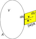
Figure "volume variation" shows a volume V bound by an area A. Over time, if the boundary A moves, the volume of V may vary. In particular, an infinitesimal area dA with outward pointing unit normal n moves with a velocity v.

This leads to a volume variation d V = d A ( v ⋅ n ) d t . Making use of Gauss's theorem, the variation in time of the total volume V volume moving in space is

The rightmost term is a volume integral over the volume V and the middle term is the surface integral over the boundary A of the volume V. Also, v is the velocity with which the points in V are moving.

In optics coordinate x 3   takes the role of time. In phase space a light ray is identified by a point ( x 1 , x 2 , p 1 , p 2 )   which moves with a "velocity" v = ( x ˙ 1 , x ˙ 2 , p ˙ 1 , p ˙ 2 )   where the dot represents a derivative relative to x 3   . A set of light rays spreading over d x 1   in coordinate x 1   , d x 2   in coordinate x 2   , d p 1   in coordinate p 1   and d p 2   in coordinate p 2   occupies a volume d V = d x 1 d x 2 d p 1 d p 2   in phase space. In general, a large set of rays occupies a large volume V   in phase space to which Gauss's theorem may be applied

and using Hamilton's equations

or d V / d x 3 = 0   and d V = d x 1 d x 2 d p 1 d p 2 = Constant   which means that the phase space volume is conserved as light travels along an optical system.

The volume occupied by a set of rays in phase space is called etendue, which is conserved as light rays progress in the optical system along direction x₃. This corresponds to Liouville's theorem, which also applies to Hamiltonian mechanics.

However, the meaning of Liouville’s theorem in mechanics is rather different from the theorem of conservation of étendue. Liouville’s theorem is essentially statistical in nature, and it refers to the evolution in time of an ensemble of mechanical systems of identical properties but with different initial conditions. Each system is represented by a single point in phase space, and the theorem states that the average density of points in phase space is constant in time. An example would be the molecules of a perfect classical gas in equilibrium in a container. Each point in phase space, which in this example has 2N dimensions, where N is the number of molecules, represents one of an ensemble of identical containers, an ensemble large enough to permit taking a statistical average of the density of representative points. Liouville’s theorem states that if all the containers remain in equilibrium, the average density of points remains constant.

Imaging and nonimaging optics

Figure "conservation of etendue" shows on the left a diagrammatic two-dimensional optical system in which x₂=0 and p₂=0 so light travels on the plane x₁x₃ in directions of increasing x₃ values.

Light rays crossing the input aperture of the optic at point x₁=x_I are contained between edge rays r_A and r_B represented by a vertical line between points r_A and r_B at the phase space of the input aperture (right, bottom corner of the figure). All rays crossing the input aperture are represented in phase space by a region R_I.

Also, light rays crossing the output aperture of the optic at point x₁=x_O are contained between edge rays r_A and r_B represented by a vertical line between points r_A and r_B at the phase space of the output aperture (right, top corner of the figure). All rays crossing the output aperture are represented in phase space by a region R_O.

Conservation of etendue in the optical system means that the volume (or area in this two-dimensional case) in phase space occupied by R_I at the input aperture must be the same as the volume in phase space occupied by R_O at the output aperture.

In imaging optics, all light rays crossing the input aperture at x₁=x_I are redirected by it towards the output aperture at x₁=x_O where x_I=m x_O. This ensures that an image of the input of formed at the output with a magnification m. In phase space, this means that vertical lines in the phase space at the input are transformed into vertical lines at the output. That would be the case of vertical line r_A r_B in R_I transformed to vertical line r_A r_B in R_O.

In nonimaging optics, the goal is not to form an image but simply to transfer all light from the input aperture to the output aperture. This is accomplished by transforming the edge rays ∂R_I of R_I to edge rays ∂R_O of R_O. This is known as the edge ray principle.

Generalizations

Above it was assumed that light travels along the x₃ axis, in Hamilton's principle above, coordinates x 1   and x 2   take the role of the generalized coordinates q k   while x 3   takes the role of parameter σ   , that is, parameter σ =x₃ and N=2. However, different parametrizations of the light rays are possible, as well as the use of generalized coordinates.

General ray parametrization

A more general situation can be considered in which the path of a light ray is parametrized as s = ( x 1 ( σ ) , x 2 ( σ ) , x 3 ( σ ) )   in which σ is a general parameter. In this case, when compared to Hamilton's principle above, coordinates x 1   , x 2   and x 3   take the role of the generalized coordinates q k   with N=3. Applying Hamilton's principle to optics in this case leads to

where now L = n d s / d σ   and x ˙ k = d x k / d σ and for which the Euler-Lagrange equations applied to this form of Fermat's principle result in

with k=1,2,3 and where L is the optical Lagrangian. Also in this case the optical momentum is defined as

and the Hamiltonian P is defined by the expression given above for N=3 corresponding to functions x 1 ( σ ) , x 2 ( σ ) and x 3 ( σ ) to be determined

And the corresponding Hamilton's equations with k=1,2,3 applied optics are

with x ˙ k = d x k / d σ and p ˙ k = d p k / d σ .

The optical Lagrangian is given by

and does not explicitly depend on parameter σ. For that reason not all solutions of the Euler-Lagrange equations will be possible light rays, since their derivation assumed an explicit dependence of L on σ which does not happen in optics.

The optical momentum components can be obtained from

where x ˙ k = d x k / d σ . The expression for the Lagrangian can be rewritten as

Comparing this expression for L with that for the Hamiltonian P it can be concluded that

From the expressions for the components p k   of the optical momentum results

The optical Hamiltonian is chosen as

although other choices could be made. The Hamilton's equations with k=1,2,3 defined above together with P = 0   define the possible light rays.

Generalized coordinates

As in Hamiltonian mechanics, it is also possible to write the equations of Hamiltonian optics in terms of generalized coordinates ( q 1 ( σ ) , q 2 ( σ ) , q 3 ( σ ) )   , generalized momenta ( u 1 ( σ ) , u 2 ( σ ) , u 3 ( σ ) )   and Hamiltonian P as

where the optical momentum is given by

and e ^ 1 , e ^ 2 and e ^ 3 are unit vectors. A particular case is obtained when these vectors form an orthonormal basis, that is, they are all perpendicular to each other. In that case, u k a k / n   is the cosine of the angle the optical momentum p makes to unit vector e ^ k .