Generalized distributive law

Introduction

"The distributive law in mathematics is the law relating the operations of multiplication and addition, stated symbolically, a ∗ ( b + c ) = a ∗ b + a ∗ c ; that is, the monomial factor a is distributed, or separately applied, to each term of the binomial factor b + c , resulting in the product a ∗ b + a ∗ c " - Britannica

As it can be observed from the definition, application of distributive law to an arithmetic expression reduces the number of operations in it. In the previous example the total number of operations reduced from three (two multiplications and an addition in a ∗ b + a ∗ c ) to two (one multiplication and one addition in a ∗ ( b + c ) ). Generalization of distributive law leads to a large family of fast algorithms. This includes the FFT and Viterbi algorithm.

This is explained in a more formal way in the example below:

α ( a , b ) = d e f ∑ c , d , e ∈ A f ( a , c , b ) g ( a , d , e ) where f ( ⋅ ) and g ( ⋅ ) are real-valued functions, a , b , c , d , e ∈ A and | A | = q (say)

Here we are "marginalizing out" the independent variables ( c , d , and e ) to obtain the result. When we are calculating the computational complexity, we can see that for each q 2 pairs of ( a , b ) , there are q 3 terms due to the triplet ( c , d , e ) which needs to take part in the evaluation of α ( a , b ) with each step having one addition and one multiplication. Therefore, the total number of computations needed is 2 ⋅ q 2 ⋅ q 3 = 2 q 5 . Hence the asymptotic complexity of the above function is O ( n 5 ) .

If we apply the distributive law to the RHS of the equation, we get the following:

This implies that α ( a , b ) can be described as a product α 1 ( a , b ) ⋅ α 2 ( a ) where α 1 ( a , b ) = d e f ∑ c ∈ A f ( a , c , b ) and α 2 ( a ) = d e f ∑ d , e ∈ A g ( a , d , e )

Now, when we are calculating the computational complexity, we can see that there are q 3 additions in α 1 ( a , b ) and α 2 ( a ) each and there are q 2 multiplications when we are using the product α 1 ( a , b ) ⋅ α 2 ( a ) to evaluate α ( a , b ) . Therefore, the total number of computations needed is q 3 + q 3 + q 2 = 2 q 3 + q 2 . Hence the asymptotic complexity of calculating α ( a , b ) reduces to O ( n 3 ) from O ( n 5 ) . This shows by an example that applying distributive law reduces the computational complexity which is one of the good features of a "fast algorithm".

History

Some of the problems that used distributive law to solve can be grouped as follows

1. Decoding algorithms
A GDL like algorithm was used by Gallager's for decoding low density parity-check codes. Based on Gallager's work Tanner introduced the Tanner graph and expressed Gallagers work in message passing form. The tanners graph also helped explain the Viterbi algorithm.

It is observed by Forney that Viterbi's maximum likelihood decoding of convolutional codes also used algorithms of GDL-like generality.

2. Forward-backward algorithm
The forward backward algorithm helped as an algorithm for tracking the states in the markov chain. And this also was used the algorithm of GDL like generality

3. Artificial intelligence
The notion of junction trees has been used to solve many problems in AI. Also the concept of bucket elimination used many of the concepts.

The MPF problem

MPF or marginalize a product function is a general computational problem which as special case includes many classical problems such as computation of discrete Hadamard transform, maximum likelihood decoding of a linear code over a memory-less channel, and matrix chain multiplication. The power of the GDL lies in the fact that it applies to situations in which additions and multiplications are generalized. A commutative semiring is a good framework for explaining this behavior. It is defined over a set K with operators " + " and " . " where ( K , + ) and ( K , . ) are a commutative monoids and the distributive law holds.

Let p 1 , … , p n be variables such that p 1 ∈ A 1 , … , p n ∈ A n where A is a finite set and | A i | = q i . Here i = 1 , … , n . If S = { i 1 , … , i r } and S ⊂ { 1 , … , n } , let A S = A i 1 × ⋯ × A i r , p S = ( p i 1 , … , p i r ) , q S = | A S | , A = A 1 × ⋯ × A n , and p = { p 1 , … , p n }

Let S = { S j } j = 1 M where S j ⊂ { 1 , . . . , n } . Suppose a function is defined as α i : A S i → R , where R is a commutative semiring. Also, p S i are named the local domains and α i as the local kernels.

Now the global kernel β : A → R is defined as : β ( p 1 , . . . , p n ) = ∏ i = 1 M α ( p S i )

Definition of MPF problem: For one or more indices i = 1 , . . . , M , compute a table of the values of S i -marginalization of the global kernel β , which is the function β i : A S i → R defined as β i ( p S i ) = ∑ p S i c ∈ A S i c β ( p )

Here S i c is the complement of S i with respect to { 1 , . . . , n } and the β i ( p S i ) is called the i t h objective function, or the objective function at S i . It can observed that the computation of the i t h objective function in the obvious way needs M q 1 q 2 q 3 ⋯ q n operations. This is because there are q 1 q 2 ⋯ q n additions and ( M − 1 ) q 1 q 2 . . . q n multiplications needed in the computation of the i th objective function. The GDL algorithm which is explained in the next section can reduce this computational complexity.

The following is an example of the MPF problem. Let p 1 , p 2 , p 3 , p 4 , and p 5 be variables such that p 1 ∈ A 1 , p 2 ∈ A 2 , p 3 ∈ A 3 , p 4 ∈ A 4 , and p 5 ∈ A 5 . Here M = 4 and S = { { 1 , 2 , 5 } , { 2 , 4 } , { 1 , 4 } , { 2 } } . The given functions using these variables are f ( p 1 , p 2 , p 5 ) and g ( p 3 , p 4 ) and we need to calculate α ( p 1 , p 4 ) and β ( p 2 ) defined as:

Here local domains and local kernels are defined as follows:

where α ( p 1 , p 4 ) is the 3 r d objective function and β ( p 2 ) is the 4 t h objective function.

Let us consider another example where p 1 , p 2 , p 3 , p 4 , r 1 , r 2 , r 3 , r 4 ∈ { 0 , 1 } and f ( r 1 , r 2 , r 3 , r 4 ) is a real valued function. Now, we shall consider the MPF problem where the commutative semiring is defined as the set of real numbers with ordinary addition and multiplication and the local domains and local kernels are defined as follows:

Now since the global kernel is defined as the product of the local kernels, it is

and the objective function at the local domain p 1 , p 2 , p 3 , p 4 is

This is the Hadamard transform of the function f ( ⋅ ) . Hence we can see that the computation of Hadamard transform is a special case of the MPF problem. More examples can be demonstrated to prove that the MPF problem forms special cases of many classical problem as explained above whose details can be found at

GDL: an algorithm for solving the MPF problem

If one can find a relationship among the elements of a given set S , then one can solve the MPF problem basing on the notion of belief propagation which is a special use of "message passing" technique. The required relationship is that the given set of local domains can be organised into a junction tree. In other words, we create a graph theoretic tree with the elements of S as the vertices of the tree T , such that for any two arbitrary vertices say v i and v j where i ≠ j and there exists an edge between these two vertices, then the intersection of corresponding labels, viz S i ∩ S j , is a subset of the label on each vertex on the unique path from v i to v j .

For example,

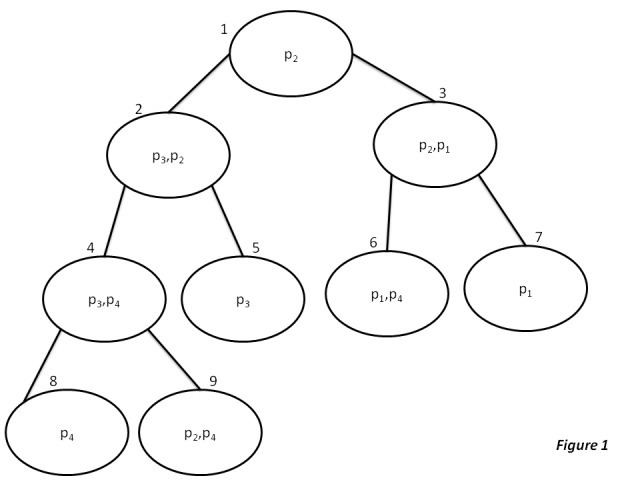
Example 1: Consider the following nine local domains:

1. { p 2 }
2. { p 3 , p 2 }
3. { p 2 , p 1 }
4. { p 3 , p 4 }
5. { p 3 }
6. { p 1 , p 4 }
7. { p 1 }
8. { p 4 }
9. { p 2 , p 4 }

For the above given set of local domains, one can organize them into a junction tree as shown below:

Similarly If another set like the following is given

Example 2: Consider the following four local domains:

1. { p 1 , p 2 }
2. { p 2 , p 3 }
3. { p 3 , p 4 }
4. { p 1 , p 4 }

Then constructing the tree only with these local domains is not possible since this set of values has no common domains which can be placed between any two values of the above set. But however if add the two dummy domains as shown below then organizing the updated set into a junction tree would be possible and easy too.

5. { p 1 , p 2 , p 4 }
6. { p 2 , p 3 , p 4 }

Similarly for these set of domains, the junction tree looks like shown below:

Generalized distributive law (GDL) algorithm

Input: A set of local domains.
Output: For the given set of domains, possible minimum number of operations that is required to solve the problem is computed.
So, if v i and v j are connected by an edge in the junction tree, then a message from v i to v j is a set/table of values given by a function: μ i , j : A S i ∩ S j → R . To begin with all the functions i.e. for all combinations of i and j in the given tree, μ i , j is defined to be identically 1 and when a particular message is update, it follows the equation given below.

where v k adj ⁡ v i means that v k is an adjacent vertex to v i in tree.

Similarly each vertex has a state which is defined as a table containing the values from the function σ i : A S i → R , Just like how messages initialize to 1 identically, state of v i is defined to be local kernel α ( p S i ) , but whenever σ i gets updated, it follows the following equation:

Basic working of the algorithm

For the given set of local domains as input, we find out if we can create a junction tree, either by using the set directly or by adding dummy domains to the set first and then creating the junction tree, if construction junction is not possible then algorithm output that there is no way to reduce the number of steps to compute the given equation problem, but once we have junction tree, algorithm will have to schedule messages and compute states, by doing these we can know where steps can be reduced, hence will be discusses this below.

Scheduling of the message passing and the state computation

There are two special cases we are going to talk about here namely Single Vertex Problem in which the objective function is computed at only one vertex v 0 and the second one is All Vertices Problem where the goal is to compute the objective function at all vertices.

Lets begin with the single-vertex problem, GDL will start by directing each edge towards the targeted vertex v 0 . Here messages are sent only in the direction towards the targeted vertex. Note that all the directed messages are sent only once. The messages are started from the leaf nodes(where the degree is 1) go up towards the target vertex v 0 . The message travels from the leaves to its parents and then from there to their parents and so on until it reaches the target vertex v 0 . The target vertex v 0 will compute its state only when it receives all messages from all its neighbors. Once we have the state, We have got the answer and hence the algorithm terminates.

For Example, Lets consider a junction tree constructed from the set of local domains given above i.e. the set from example 1,
Now the Scheduling table for these domains is (where the target vertex is p 2 ).

Round Message or State Computation
1. μ 8 , 4 ( p 4 ) = α 8 ( p 4 )
2. μ 8 , 4 ( p 4 ) = Σ p 2 α 9 ( p 2 , p 4 )
3. μ 5 , 2 ( p 3 ) = α 5 ( p 3 )
4. μ 6 , 3 ( p 1 ) = Σ p 4 α 6 ( p 1 , p 4 )
5. μ 7 , 3 ( p 1 ) = α 7 ( p 1 )
6. μ 4 , 2 ( p 3 ) = Σ p 4 α 4 ( p 3 , p 4 ) . μ 8 , 4 ( p 4 ) . μ 9 , 4 ( p 4 )
7. μ 3 , 1 ( p 2 ) = Σ p 1 α 3 ( p 2 , p 1 ) . μ 6 , 3 ( p 1 ) . μ 7 , 3 ( p 1 )
8. μ 2 , 1 ( p 2 ) = Σ p 3 α 2 ( p 3 , p 2 ) . μ 4 , 2 ( p 3 ) . μ 5 , 2 ( p 3 )
9. σ 1 ( p 2 ) = α 1 ( p 2 ) . μ 2 , 1 ( p 2 ) . μ 3 , 1 ( p 2 )

Thus the complexity for Single Vertex GDL can be shown as

Σ v d ( v ) | A S ( v ) | arithmetic operations
Where (Note: The explanation for the above equation is explained later in the article )
S ( v ) is the label of v .
d ( v ) is the degree of v (i.e. number of vertices adjacent to v).

To solve the All-Vertices problem, we can schedule GDL in several ways, some of them are parallel implementation where in each round, every state is updated and every message is computed and transmitted at the same time. In this type of implementation the states and messages will stabilizes after number of rounds that is at most equal to the diameter of the tree. At this point all the all states of the vertices will be equal to the desired objective function.

Another way to schedule GDL for this problem is serial implementation where its similar to the Single vertex problem except that we don't stop the algorithm until all the vertices of a required set have not got all the messages from all their neighbors and have compute their state.
Thus the number of arithmetic this implementation requires is at most Σ v ∈ V d ( v ) | A S ( v ) | arithmetic operations.

Constructing a junction tree

The key to constructing a junction tree lies in the local domain graph G L D , which is a weighted complete graph with M vertices v 1 , v 2 , v 3 , … , v M i.e. one for each local domain, having the weight of the edge e i , j : v i ↔ v j defined by
ω i , j = | S i ∩ S j | .
if x k ∈ S i ∩ S j , then we say x k is contained in e i , j . Denoted by ω m a x (the weight of a maximal-weight spanning tree of G L D ), which is defined by

where n is the number of elements in that set. For more clarity and details, please refer to these.

Scheduling theorem

Let ′ T ′ be a junction tree with vertex set ′ V ′ and edge set ′ E ′ . In this algorithm, the messages are sent in both the direction on any edge, so we can say/regard the edge set E as set of ordered pairs of vertices. For example, from Figure 1 ′ E ′ can be defined as follows

NOTE: E above gives you all the possible directions that a message can travel in the tree.

The schedule for the GDL is defined as a finite sequence of subsets of E . Which is generally represented by E = { E 1 , E 2 , E 3 , … , E N }, Where E N is the set of messages updated during the N t h round of running the algorithm.

Having defined/seen some notations, we will see want the theorem says, When we are given a schedule E = { E 1 , E 2 , E 3 , … , E N } , the corresponding message trellis as a finite directed graph with Vertex set of V × { 0 , 1 , 2 , 3 , … , N } , in which a typical element is denoted by v i ( t ) for t ∈ { 0 , 1 , 2 , 3 , … , N } , Then after completion of the message passing, state at vertex v j will be the j th objective defined in

and iff there is a path from v i ( 0 ) to v j ( N )

Computational complexity

Here we try to explain the complexity of solving the MPF problem in terms of the number of mathematical operations required for the calculation. i.e. We compare the number of operations required when calculated using the normal method (Here by normal method we mean by methods that do not use message passing or junction trees in short methods that do not use the concepts of GDL)and the number of operations using the generalized distributive law.

Example: Let us consider the simplest case where we need to compute the following expression a b + a c .

To evaluate this expression naively requires two multiplications and one addition. The expression when expressed using the distributive law can be written as a ( b + c ) a simple optimization that reduces the number of operations to one addition and one multiplication.

Similar to the above explained example we will be expressing the equations in different forms to perform as few operation as possible by applying the GDL.

As explained in the previous sections we solve the problem by using the concept of the junction trees. The optimization obtained by the use of these trees is comparable to the optimization obtained by solving a semi group problem on trees. For example, to find the minimum of a group of numbers we can observe that if we have a tree and the elements are all at the bottom of the tree, then we can compare the minimum of two items in parallel and the resultant minimum will be written to the parent. When this process is propagated up the tree the minimum of the group of elements will be found at the root.

The following is the complexity for solving the junction tree using message passing

We rewrite the formula used earlier to the following form. This is the eqn for a message to be sent from vertex v to w

Similarly we rewrite the equation for calculating the state of vertex v as follows

We first will analyze for the single-vertex problem and assume the target vertex is v 0 and hence we have one edge from v to v 0 . Suppose we have an edge ( v , w ) we calculate the message using the message equation. To calculate p u ∩ v requires

additions and

multiplications.

(We represent the | A S ( v )   S ( w ) | as q v ∖ w .)

But there will be many possibilities for x v ∩ w hence
q v ∩ w = d e f | A S ( v ) ∩ S ( w ) | possibilities for p v ∩ w . Thus the entire message will need

additions and

multiplications

The total number of arithmetic operations required to send a message towards v 0 along the edges of tree will be

additions and

multiplications.

Once all the messages have been transmitted the algorithm terminates with the computation of state at v 0 The state computation requires d ( v 0 ) q 0 more multiplications. Thus number of calculations required to calculate the state is given as below

additions and

multiplications

Thus the grand total of the number of calculations is

where e = ( v , w ) is an edge and its size is defined by q v ∩ w

The formula above gives us the upper bound.

If we define the complexity of the edge e = ( v , w ) as

Therefore, ( 1 ) can be written as

We now calculate the edge complexity for the problem defined in Figure 1 as follows

The total complexity will be 3 q 2 q 3 + 3 q 3 q 4 + 3 q 1 q 2 + q 2 q 4 + q 1 q 4 − q 1 − q 3 − q 4 which is considerably low compared to the direct method. (Here by direct method we mean by methods that do not use message passing. The time taken using the direct method will be the equivalent to calculating message at each node and time to calculate the state of each of the nodes.)

Now we consider the all-vertex problem where the message will have to be sent in both the directions and state must be computed at both the vertexes. This would take O ( ∑ v d ( v ) d ( v ) q v ) but by precomputing we can reduce the number of multiplications to 3 ( d − 2 ) . Here d is the degree of the vertex. Ex : If there is a set ( a 1 , … , a d ) with d numbers. It is possible to compute all the d products of d − 1 of the a i with at most 3 ( d − 2 ) multiplications rather than the obvious d ( d − 2 ) . We do this by precomputing the quantities b 1 = a 1 , b 2 = b 1 ⋅ a 2 = a 1 ⋅ a 2 , b d − 1 = b d − 2 ⋅ a d − 1 = a 1 a 2 ⋯ a d − 1 and c d = a d , c d − 1 = a d − 1 c d = a d − 1 ⋅ a d , … , c 2 = a 2 ⋅ c 3 = a 2 a 3 ⋯ a d this takes 2 ( d − 2 ) multiplications. Then if m j denotes the product of all a i except for a j we have m 1 = c 2 , m 2 = b 1 ⋅ c 3 and so on will need another d − 2 multiplications making the total 3 ( d − 2 )

There is not much we can do when it comes to the construction of the junction tree except that we may have many maximal weight spanning tree and we should choose the spanning tree with the least χ ( T ) and sometimes this might mean adding a local domain to lower the junction tree complexity.

It may seem that GDL is correct only when the local domains can be expressed as a junction tree. But even in cases where there are cycles and a number of iterations the messages will approximately be equal to the objective function. The experiments on Gallager–Tanner–Wiberg algorithm for low density parity-check codes were supportive of this claim.