
 | ||
The Gabor transform, named after Dennis Gabor, is a special case of the short-time Fourier transform. It is used to determine the sinusoidal frequency and phase content of local sections of a signal as it changes over time. The function to be transformed is first multiplied by a Gaussian function, which can be regarded as a window function, and the resulting function is then transformed with a Fourier transform to derive the time-frequency analysis. The window function means that the signal near the time being analyzed will have higher weight. The Gabor transform of a signal x(t) is defined by this formula:
Contents
- Inverse Gabor transform
- Properties of the Gabor transform
- Application and example
- Discrete Gabor transformation
- References
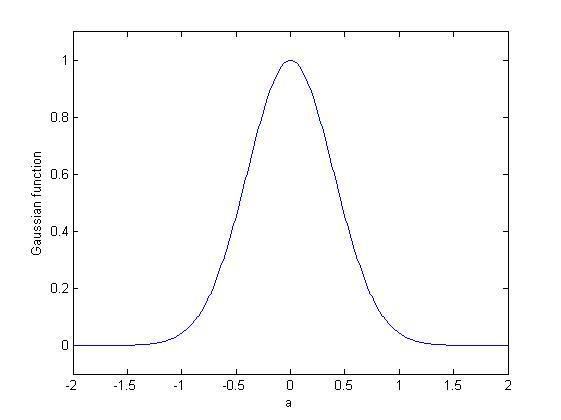
The Gaussian function has infinite range and it is impractical for implementation. However, a level of significance can be chosen (for instance 0.00001) for the distribution of the Gaussian function.
Outside these limits of integration (
This simplification makes the Gabor transform practical and realizable.
The window function width can also be varied to optimize the time-frequency resolution tradeoff for a particular application by replacing the
Inverse Gabor transform
The Gabor transform is invertible. The original signal can be recovered by the following equation
Compare this inversion formula with property No. 5 below.
Properties of the Gabor transform
The Gabor transform has many properties like those of the Fourier transform. These properties are listed in the following tables.
Application and example
The main application of the Gabor transform is used in time–frequency analysis. Take the following equation as an example. The input signal has 1 Hz frequency component when t ≤ 0 and has 2 Hz frequency component when t > 0
But if the total bandwidth available is 5 Hz, other frequency bands except x(t) are wasted. Through time–frequency analysis by applying the Gabor transform, the available bandwidth can be known and those frequency bands can be used for other applications and bandwidth is saved. The right side picture shows the input signal x(t) and the output of the Gabor transform. As was our expectation, the frequency distribution can be separated into two parts. One is t ≤ 0 and the other is t > 0. The white part is the frequency band occupied by x(t) and the black part is not used. Note that for each point in time there is both a negative (upper white part) and a positive (lower white part) frequency component.
Discrete Gabor-transformation
A discrete version of Gabor representation
with
can be derived easily by discretizing the Gabor-basis-function in these equations. Hereby the continuous parameter t is replaced by the discrete time k. Furthermore the now finite summation limit in Gabor representation has to be considered. In this way, the sampled signal y(k) is split into M time frames of length N. According to
Similar to the DFT (discrete Fourier transformation) a frequency domain split into N discrete partitions is obtained. An inverse transformation of these N spectral partitions then leads to N values y(k)for the time window, which consists of N sample values. For overall M time windows with N sample values, each signal y(k) contains K=N
with
According to the equation above, the N
For over-sampling