
 | ||
In probability theory, fractional Brownian motion (fBm), also called a fractal Brownian motion, is a generalization of Brownian motion. Unlike classical Brownian motion, the increments of fBm need not be independent. fBm is a continuous-time Gaussian process BH(t) on [0, T], which starts at zero, has expectation zero for all t in [0, T], and has the following covariance function:
Contents
- Background and definition
- Self similarity
- Stationary increments
- Long range dependence
- Regularity
- Dimension
- Integration
- Frequency domain interpretation
- Sample paths
- Method 1 of simulation
- Method 2 of simulation
- References
where H is a real number in (0, 1), called the Hurst index or Hurst parameter associated with the fractional Brownian motion. The Hurst exponent describes the raggedness of the resultant motion, with a higher value leading to a smoother motion. It was introduced by Mandelbrot & van Ness (1968).
The value of H determines what kind of process the fBm is:
The increment process, X(t) = BH(t+1) − BH(t), is known as fractional Gaussian noise.
There is also a generalization of fractional Brownian motion: n-th order fractional Brownian motion, abbreviated as n-fBm. n-fBm is a Gaussian, self-similar, non-stationary process whose increments of order n are stationary. For n = 1, n-fBm is classical fBm.
Like the Brownian motion that it generalizes, fractional Brownian motion is named after 19th century biologist Robert Brown; fractional Gaussian noise is named after mathematician Carl Friedrich Gauss.
Background and definition
Prior to the introduction of the fractional Brownian motion, Lévy (1953) used the Riemann–Liouville fractional integral to define the process
where integration is with respect to the white noise measure dB(s). This integral turns out to be ill-suited to applications of fractional Brownian motion because of its over-emphasis of the origin (Mandelbrot & van Ness 1968, p. 424).
The idea instead is to use a different fractional integral of white noise to define the process: the Weyl integral
for t > 0 (and similarly for t < 0).
The main difference between fractional Brownian motion and regular Brownian motion is that while the increments in Brownian Motion are independent, the opposite is true for fractional Brownian motion. This dependence means that if there is an increasing pattern in the previous steps, then it is likely that the current step will be increasing as well. (If H > 1/2.)
Self-similarity
The process is self-similar, since in terms of probability distributions:
This property is due to the fact that the covariance function is homogeneous of order 2H and can be considered as a fractal property. Fractional Brownian motion is the only self-similar Gaussian process.
Stationary increments
It has stationary increments:
Long-range dependence
For H > ½ the process exhibits long-range dependence,
Regularity
Sample-paths are almost nowhere differentiable. However, almost-all trajectories are Hölder continuous of any order strictly less than H: for each such trajectory, for every T > 0 and for every ε > 0 there exists a constant c such that
for 0 < s,t < T.
Dimension
With probability 1, the graph of BH(t) has both Hausdorff dimension and box dimension of 2−H.
Integration
As for regular Brownian motion, one can define stochastic integrals with respect to fractional Brownian motion, usually called "fractional stochastic integrals". In general though, unlike integrals with respect to regular Brownian motion, fractional stochastic integrals are not semimartingales.
Frequency-domain interpretation
Just as Brownian motion can be viewed as white noise filtered by
Sample paths
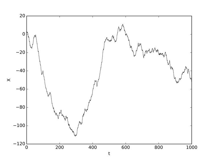
Practical computer realisations of an fBm can be generated, although they are only a finite approximation. The sample paths chosen can be thought of as showing discrete sampled points on an fBm process. Three realisations are shown below, each with 1000 points of an fBm with Hurst parameter 0.75.
Two realisations are shown below, each showing 1000 points of an fBm, the first with Hurst parameter 0.15, the second with Hurst parameter 0.55, and the third with Hurst parameter 0.95. The higher Hurst parameter is, the more smooth the curve will be.
Method 1 of simulation
One can simulate sample-paths of an fBm using methods for generating stationary Gaussian processes with known covariance function. The simplest method relies on the Cholesky decomposition method of the covariance matrix (explained below), which on a grid of size
Suppose we want to simulate the values of the fBM at times
In order to compute
Note that the result is real-valued because
Note that since the eigenvectors are linearly independent, the matrix
Method 2 of simulation
It is also known that
where B is a standard Brownian motion and
Where
Say we want simulate an fBm at points
The integral may be efficiently computed by Gaussian quadrature. Hypergeometric functions are part of the GNU scientific library.