
 | ||
The magnetocrystalline anisotropy energy of a ferromagnetic crystal can be expressed as a power series of direction cosines of the magnetic moment with respect to the crystal axes. The coefficient of those terms are the anisotropy constant. In general the expansion is limited to few terms. Normally the magnetization curve is continuous respect to applied field up to saturation but, in certain intervals of the anisotropy constant values, irreversible field induced rotations of the magnetization are possible implying first order magnetization transition between equivalent magnetization minima, the so-called first order magnetization process (FOMP).
Contents
Theory
The total energy of an uniaxial magnetic crystal in an applied magnetic field can be written as a summation of the anisotropy term up to six order, neglecting the sixfold planar contribution,
and the field dependent Zeeman energy term
where:
so the total energy can be written
Phase diagram of easy and hard directions
In order to determine the preferred directions the magnetization vector in the absence of the external magnetic field we analyze first the case of uniaxial crystal. The maxima and minima of energy with respect to θ must satisfy
while for the existence of the minima
For symmetry reasons the c-axis (θ=0) and the basal plane (θ=π/2) are always points of extrema and can be easy or hard directions depending on the anisotropy constant values. We can have two additional extrema along conical directions at angles given by:
The C + and C − are the cones associated to the + and - sign. It can be verified that the only C + is always a minimum and can be an easy direction, while C − is always a hard direction.
A useful representation of the diagram of the easy directions and other extrema is the representation in term of reduced anisotropy constant K2 / K1 and K3 / K1 . The following figure shows the phase diagram for the two cases K1>0 and K1<0 . All the information concerning the easy directions and the other extrema are contained in a special symbol that marks every different region. It simulate a polar type of energy representation indicating existing extrema by concave (minimum) and convex tips (maximum). Vertical and horizontal stems refer to the symmetry axis and the basal plane respectively. The left-hand and the right-hand oblique stems indicate the C − and C + cones respectively. The absolute minimum (easy direction) is indicated by filling of the tip.
The K ⇌ R {\displaystyle K\rightleftharpoons R} transformation
Before going into the details of the calculation of the various types of FOMP we call the readers attention to a convenient transformation of the anisotropy constants K1 , K2 , K3 into conjugate quantities, denoted by R1 , R2 , R3 . This transformation can be found in such a way that all the results obtained for the case of H parallel to c-axis can be immediately transferred to the case of H perpendicular to c-axis and vice versa according to the following symmetrical dual correspondence:
The use of the table is very simple. If we have a magnetization curve obtained with H perpendicular to c-axis and with the anisotropy constant K1, K2, K3 , we can have exactly the same magnetization curve using R1, R2, R3 according to the table but applying the H parallel to c-axis and vice versa.
FOMP examples
The determination of the conditions for the existence of FOMP requires the analysis of the magnetization curve dependence on the anisotropy constant values, for different directions of the magnetic field. We limit the analysis to the cases for H parallel or perpendicular to the c-axis, hereafter indicated as A-case and P-case, where A denotes axial while P stands for planar. The analysis of the equilibrium conditions shows that two types of FOMP are possible, depending on the final state after the transition, in case of saturation we have (type-1 FOMP) otherwise (type-2 FOMP). In the case when an easy cone is present we add the suffix C to the description of the FOMP-type. So all possible cases of FOMP-type are: A1, A2, P1, P2, P1C, A1C. In the following figure some examples of FOMP-type are represented, i.e. P1, A1C and P2 for different anisotropy constants, reduced variable are given on the axes, in particular on the abscissa h=Ms/|K1| and on the ordinate m=M/Ms.
FOMP diagram
Tedious calculations allow now to determine completely the regions of existence of type 1 or type 2 FOMP. As in the case of the diagram of the easy directions and other extrema is convenient the representation in term of reduced anisotropy constant K2 / K1 and K3 / K1 . In the following figure we summarize all the FOMP-types distinguished by the labels A1, A2, P1, P2, P1C, A1C which specifies the magnetic field directions (A axial; P planar) and the type of FOMP (1 and 2) and the easy cone regions with type 1 FOMP (A1C, P1C).
Polycrystalline system
Since the FOMP transition represents a singular point in the magnetization curve of a single crystal, we analyze how this singularity is transformed when we magnetize a polycrystalline sample. The result of the mathematical analysis shows the possibility of carrying out the measurement of critical field ( Hcr ) where the FOMP transition takes place in the case of polycrystalline samples.
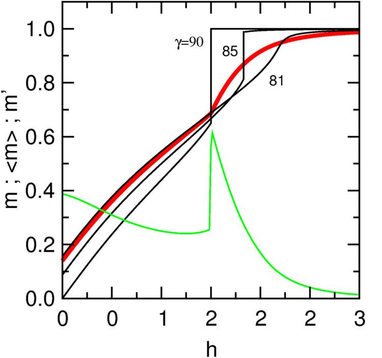
For determining the characteristics of FOMP when the magnetic field is applied at a variable angle γ with respect to the c axis, we have to examine the evolution of the total energy of the crystal with increasing field for different values of γ between 0 and π/2. The calculations are complicated and we report only the conclusions. The sharp FOMP transition, evident in single crystal, in the case of polycrystalline samples moves at higher fields for H different from hard direction and then becomes smeared out. For higher value of γ the magnetization curve becomes smooth, as is evident from computer magnetization curves obtained by summation of all curves corresponding to all angles γ between 0 and π/2.
Origin of high order anisotropy constants
The origin of high anisotropy constant can be found in the interaction of two sublattices (A and B) each of them having a competing high anisotropy energy, i.e. having different easy directions. In particular we can no longer consider the system as a rigid collinear magnetic structure, but we must allow for substantial deviations from the equilibrium configuration present at zero field. Limiting up to fourth order, neglecting the in plane contribution, the anisotropy energy becomes:
where:
The equilibrium equation of the anisotropy energy has not a complete analytical solution so computer analysis is useful. The interesting aspect regards the simulation of the resulted magnetization curves, analytical or discontinuous with FOMP. By computer it is possible to fit the obtained results by an equivalent anisotropy energy expression:
where:
So starting from a forth order anisotropy energy expression we obtain an equivalent expression of sixth order, that is higher anisotropy constant can be derived from the competing anisotropy of different sublattices.
FOMP in other symmetries
The problem for cubic crystal system has been approached by Bozorth, and partial results have been obtained by different authors, but exact complete phase diagrams with anisotropy contributions up to sixth and eighth order have only been determined more recently.
The FOMP in the trigonal crystal system has been analyzed for case of the anisotropy energy expression up to forth order:
where θ and φ are the polar angles of the magnetization vector with respect to c-axis. The study of the energy derivatives allows the determination of the magnetic phase and the FOMP-phase as in the hexagonal case, see the reference for the diagrams.