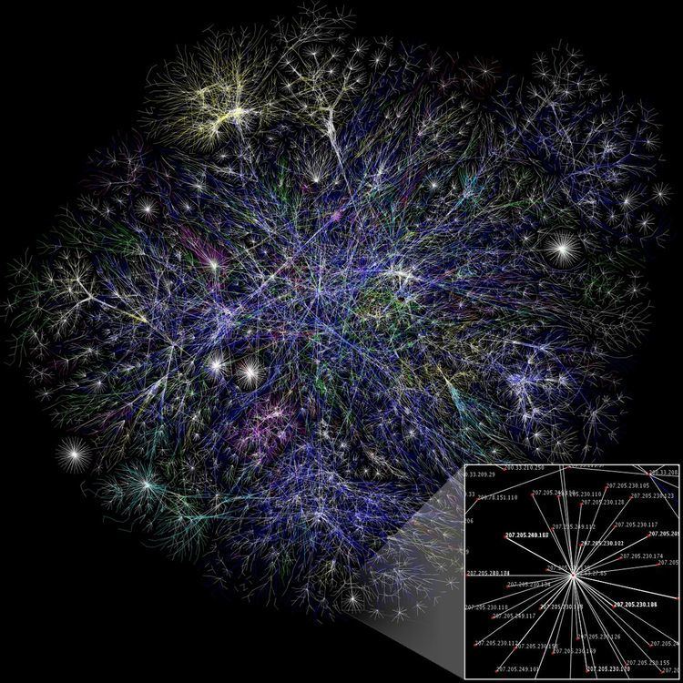
 | ||
In graph theory, the Erdős–Rényi model is either of two closely related models for generating random graphs. They are named after Paul Erdős and Alfréd Rényi, who first introduced one of the models in 1959; the other model was introduced independently and contemporaneously by Edgar Gilbert. In the model introduced by Erdős and Rényi, all graphs on a fixed vertex set with a fixed number of edges are equally likely; in the model introduced by Gilbert, each edge has a fixed probability of being present or absent, independently of the other edges. These models can be used in the probabilistic method to prove the existence of graphs satisfying various properties, or to provide a rigorous definition of what it means for a property to hold for almost all graphs.
Contents
Definition
There are two closely related variants of the Erdős–Rényi (ER) random graph model.
The behavior of random graphs are often studied in the case where n, the number of vertices, tends to infinity. Although p and M can be fixed in this case, they can also be functions depending on n. For example, the statement
Almost every graph in G(n, 2ln(n)/n) is connected.means
As n tends to infinity, the probability that a graph on n vertices with edge probability 2ln(n)/n is connected, tends to 1.Comparison between the two models
The expected number of edges in G(n, p) is
For many graph properties, this is the case. If P is any graph property which is monotone with respect to the subgraph ordering (meaning that if A is a subgraph of B and A satisfies P, then B will satisfy P as well), then the statements "P holds for almost all graphs in G(n, p)" and "P holds for almost all graphs in
In practice, the G(n, p) model is the one more commonly used today, in part due to the ease of analysis allowed by the independence of the edges.
Properties of G(n, p)
With the notation above, a graph in G(n, p) has on average
where n is the total number of vertices in the graph. Since
this distribution is Poisson for large n and np = const.
In a 1960 paper, Erdős and Rényi described the behavior of G(n, p) very precisely for various values of p. Their results included that:
Thus
Further properties of the graph can be described almost precisely as n tends to infinity. For example, there is a k(n) (approximately equal to 2log2(n)) such that the largest clique in G(n, 0.5) has almost surely either size k(n) or k(n) + 1.
Thus, even though finding the size of the largest clique in a graph is NP-complete, the size of the largest clique in a "typical" graph (according to this model) is very well understood.
Interestingly, edge-dual graphs of Erdos-Renyi graphs are graphs with nearly the same degree distribution, but with degree correlations and a significantly higher clustering coefficient.
Relation to percolation
In percolation theory one examines a finite or infinite graph and removes edges (or links) randomly. Thus the Erdős–Rényi process is in fact unweighted link percolation on the complete graph. (One refers to percolation in which nodes and/or links are removed with heterogeneous weights as weighted percolation). As percolation theory has much of its roots in physics, much of the research done was on the lattices in Euclidean spaces. The transition at np = 1 from giant component to small component has analogs for these graphs, but for lattices the transition point is difficult to determine. Physicists often refer to study of the complete graph as a mean field theory. Thus the Erdős–Rényi process is the mean-field case of percolation.
Some significant work was also done on percolation on random graphs. From a physicist's point of view this would still be a mean-field model, so the justification of the research is often formulated in terms of the robustness of the graph, viewed as a communication network. Given a random graph of n ≫ 1 nodes with an average degree <k>. Remove randomly a fraction 1 − p′ of nodes and leave only a fraction p′ from the network. There exists a critical percolation threshold
Caveats
Both of the two major assumptions of the G(n, p) model (that edges are independent and that each edge is equally likely) may be inappropriate for modeling certain real-life phenomena. In particular, an Erdős–Rényi graph does not have heavy tails (clarification: Consider the function f(x) with x being the degree of a vertex and f(x)=y being the number of vertices in the graph that have degree x. For an Erdős–Rényi graph this function has a horizontal asymptote at y=0, but for naturally occurring phenomena this function does not have an asymptote at y=0), as is the case in many real networks. Moreover, it has low clustering, unlike many social networks. For popular modeling alternatives, see Barabási–Albert model and Watts and Strogatz model. One should note that these alternative models are not percolation processes, but instead represent a growth and rewiring model, respectively. A model for interacting ER networks was developed recently by Buldyrev et al..
History
The G(n, p) model was first introduced by Edgar Gilbert in a 1959 paper studying the connectivity threshold mentioned above. The G(n, M) model was introduced by Erdős and Rényi in their 1959 paper. As with Gilbert, their first investigations were as to the connectivity of G(n, M), with the more detailed analysis following in 1960.
