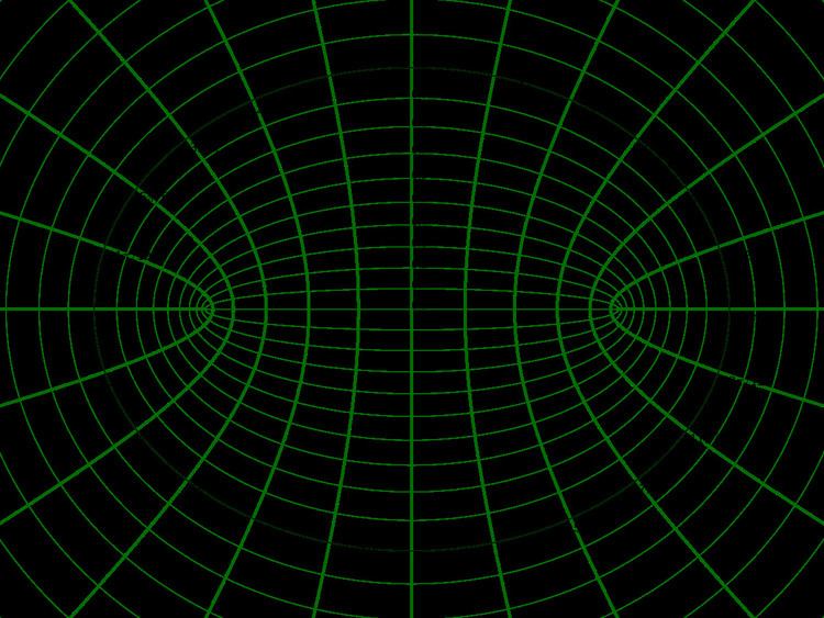
The most common definition of elliptic coordinates ( μ , ν ) is
x = a cosh μ cos ν y = a sinh μ sin ν where μ is a nonnegative real number and ν ∈ [ 0 , 2 π ] .
On the complex plane, an equivalent relationship is
x + i y = a cosh ( μ + i ν ) These definitions correspond to ellipses and hyperbolae. The trigonometric identity
x 2 a 2 cosh 2 μ + y 2 a 2 sinh 2 μ = cos 2 ν + sin 2 ν = 1 shows that curves of constant μ form ellipses, whereas the hyperbolic trigonometric identity
x 2 a 2 cos 2 ν − y 2 a 2 sin 2 ν = cosh 2 μ − sinh 2 μ = 1 shows that curves of constant ν form hyperbolae.
In an orthogonal coordinate system the lengths of the basis vectors are known as scale factors. The scale factors for the elliptic coordinates ( μ , ν ) are equal to
h μ = h ν = a sinh 2 μ + sin 2 ν = a cosh 2 μ − cos 2 ν . Using the double argument identities for hyperbolic functions and trigonometric functions, the scale factors can be equivalently expressed as
h μ = h ν = a 1 2 ( cosh 2 μ − cos 2 ν ) . Consequently, an infinitesimal element of area equals
d A = h μ h ν d μ d ν = a 2 ( sinh 2 μ + sin 2 ν ) d μ d ν = a 2 ( cosh 2 μ − cos 2 ν ) d μ d ν = a 2 2 ( cosh 2 μ − cos 2 ν ) d μ d ν and the Laplacian reads
∇ 2 Φ = 1 a 2 ( sinh 2 μ + sin 2 ν ) ( ∂ 2 Φ ∂ μ 2 + ∂ 2 Φ ∂ ν 2 ) = 1 a 2 ( cosh 2 μ − cos 2 ν ) ( ∂ 2 Φ ∂ μ 2 + ∂ 2 Φ ∂ ν 2 ) = 2 a 2 ( cosh 2 μ − cos 2 ν ) ( ∂ 2 Φ ∂ μ 2 + ∂ 2 Φ ∂ ν 2 ) . Other differential operators such as ∇ ⋅ F and ∇ × F can be expressed in the coordinates ( μ , ν ) by substituting the scale factors into the general formulae found in orthogonal coordinates.
An alternative and geometrically intuitive set of elliptic coordinates ( σ , τ ) are sometimes used, where σ = cosh μ and τ = cos ν . Hence, the curves of constant σ are ellipses, whereas the curves of constant τ are hyperbolae. The coordinate τ must belong to the interval [-1, 1], whereas the σ coordinate must be greater than or equal to one.
The coordinates ( σ , τ ) have a simple relation to the distances to the foci F 1 and F 2 . For any point in the plane, the sum d 1 + d 2 of its distances to the foci equals 2 a σ , whereas their difference d 1 − d 2 equals 2 a τ . Thus, the distance to F 1 is a ( σ + τ ) , whereas the distance to F 2 is a ( σ − τ ) . (Recall that F 1 and F 2 are located at x = − a and x = + a , respectively.)
A drawback of these coordinates is that the points with Cartesian coordinates (x,y) and (x,-y) have the same coordinates ( σ , τ ) , so the conversion to Cartesian coordinates is not a function, but a multifunction.
x = a σ τ y 2 = a 2 ( σ 2 − 1 ) ( 1 − τ 2 ) . The scale factors for the alternative elliptic coordinates ( σ , τ ) are
h σ = a σ 2 − τ 2 σ 2 − 1 h τ = a σ 2 − τ 2 1 − τ 2 . Hence, the infinitesimal area element becomes
d A = a 2 σ 2 − τ 2 ( σ 2 − 1 ) ( 1 − τ 2 ) d σ d τ and the Laplacian equals
∇ 2 Φ = 1 a 2 ( σ 2 − τ 2 ) [ σ 2 − 1 ∂ ∂ σ ( σ 2 − 1 ∂ Φ ∂ σ ) + 1 − τ 2 ∂ ∂ τ ( 1 − τ 2 ∂ Φ ∂ τ ) ] . Other differential operators such as ∇ ⋅ F and ∇ × F can be expressed in the coordinates ( σ , τ ) by substituting the scale factors into the general formulae found in orthogonal coordinates.
Elliptic coordinates form the basis for several sets of three-dimensional orthogonal coordinates. The elliptic cylindrical coordinates are produced by projecting in the z -direction. The prolate spheroidal coordinates are produced by rotating the elliptic coordinates about the x -axis, i.e., the axis connecting the foci, whereas the oblate spheroidal coordinates are produced by rotating the elliptic coordinates about the y -axis, i.e., the axis separating the foci.
The classic applications of elliptic coordinates are in solving partial differential equations, e.g., Laplace's equation or the Helmholtz equation, for which elliptic coordinates are a natural description of a system thus allowing a separation of variables in the partial differential equations. Some traditional examples are solving systems such as electrons orbiting a molecule or planetary orbits that have an elliptical shape.
The geometric properties of elliptic coordinates can also be useful. A typical example might involve an integration over all pairs of vectors p and q that sum to a fixed vector r = p + q , where the integrand was a function of the vector lengths | p | and | q | . (In such a case, one would position r between the two foci and aligned with the x -axis, i.e., r = 2 a x ^ .) For concreteness, r , p and q could represent the momenta of a particle and its decomposition products, respectively, and the integrand might involve the kinetic energies of the products (which are proportional to the squared lengths of the momenta).