Oblate spheroidal coordinates

Definition (μ, ν, φ)

The most common definition of oblate spheroidal coordinates (μ, ν, φ) is

x = a   cosh ⁡ μ   cos ⁡ ν   cos ⁡ ϕ y = a   cosh ⁡ μ   cos ⁡ ν   sin ⁡ ϕ z = a   sinh ⁡ μ   sin ⁡ ν

where μ is a nonnegative real number and the angle ν lies between ±90°. The azimuthal angle φ can fall anywhere on a full circle, between ±180°. These coordinates are favored over the alternatives below because they are not degenerate; the set of coordinates (μ, ν, φ) describes a unique point in Cartesian coordinates (x, y, z). The reverse is also true, except on the z-axis and the disk in the x-y plane inside the focal ring.

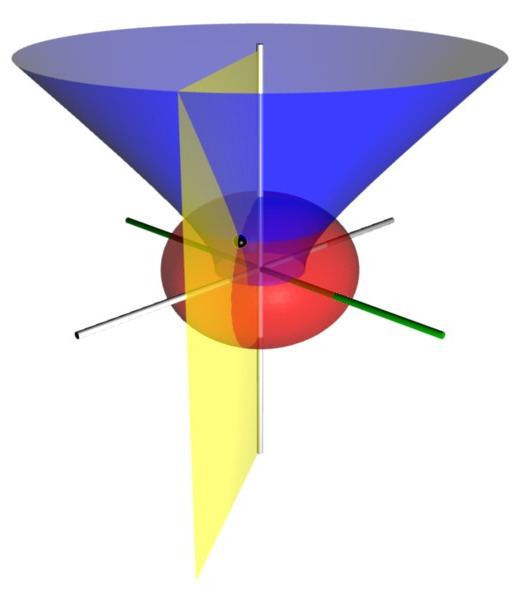
Coordinate surfaces

The surfaces of constant μ form oblate spheroids, by the trigonometric identity

x 2 + y 2 a 2 cosh 2 ⁡ μ + z 2 a 2 sinh 2 ⁡ μ = cos 2 ⁡ ν + sin 2 ⁡ ν = 1

since they are ellipses rotated about the z-axis, which separates their foci. An ellipse in the x-z plane (Figure 2) has a major semiaxis of length a cosh μ along the x-axis, whereas its minor semiaxis has length a sinh μ along the z-axis. The foci of all the ellipses in the x-z plane are located on the x-axis at ±a.

Similarly, the surfaces of constant ν form one-sheet half hyperboloids of revolution by the hyperbolic trigonometric identity

x 2 + y 2 a 2 cos 2 ⁡ ν − z 2 a 2 sin 2 ⁡ ν = cosh 2 ⁡ μ − sinh 2 ⁡ μ = 1

For positive ν, the half-hyperboloid is above the x-y plane (i.e., has positive z) whereas for negative ν, the half-hyperboloid is below the x-y plane (i.e., has negative z). Geometrically, the angle ν corresponds to the angle of the asymptotes of the hyperbola. The foci of all the hyperbolae are likewise located on the x-axis at ±a.

Inverse transformation

The (μ, ν, φ) coordinates may be calculated from the Cartesian coordinates (x, y, z) as follows. The azimuthal angle φ is given by the formula

tan ⁡ ϕ = y x

The cylindrical radius ρ of the point P is given by

ρ 2 = x 2 + y 2

and its distances to the foci in the plane defined by φ is given by

d 1 2 = ( ρ + a ) 2 + z 2 d 2 2 = ( ρ − a ) 2 + z 2

The remaining coordinates μ and ν can be calculated from the equations

cosh ⁡ μ = d 1 + d 2 2 a cos ⁡ ν = d 1 − d 2 2 a

where the sign of μ is always non-negative, and the sign of ν is the same as that of z.

Another method to compute the inverse transform is

μ = Re ⁡ arccosh ⁡ ρ + z i a ν = Im ⁡ arccosh ⁡ ρ + z i a ϕ = arctan ⁡ y x

where

ρ = x 2 + y 2

Scale factors

The scale factors for the coordinates μ and ν are equal

h μ = h ν = a sinh 2 ⁡ μ + sin 2 ⁡ ν

whereas the azimuthal scale factor equals

h ϕ = a cosh ⁡ μ   cos ⁡ ν

Consequently, an infinitesimal volume element equals

d V = a 3 cosh ⁡ μ   cos ⁡ ν   ( sinh 2 ⁡ μ + sin 2 ⁡ ν ) d μ d ν d ϕ

and the Laplacian can be written

∇ 2 Φ = 1 a 2 ( sinh 2 ⁡ μ + sin 2 ⁡ ν ) [ 1 cosh ⁡ μ ∂ ∂ μ ( cosh ⁡ μ ∂ Φ ∂ μ ) + 1 cos ⁡ ν ∂ ∂ ν ( cos ⁡ ν ∂ Φ ∂ ν ) ] + 1 a 2 cosh 2 ⁡ μ cos 2 ⁡ ν ∂ 2 Φ ∂ ϕ 2

Other differential operators such as ∇ ⋅ F and ∇ × F can be expressed in the coordinates (μ, ν, φ) by substituting the scale factors into the general formulae found in orthogonal coordinates.

Basis Vectors

The orthonormal basis vectors for the μ , ν , ϕ coordinate system can be expressed in Cartesian coordinates as

e ^ μ = 1 sinh 2 ⁡ μ + sin 2 ⁡ ν ( sinh ⁡ μ cos ⁡ ν cos ⁡ ϕ i ^ + sinh ⁡ μ cos ⁡ ν sin ⁡ ϕ j ^ + cosh ⁡ μ sin ⁡ ν k ^ ) e ^ ν = 1 sinh 2 ⁡ μ + sin 2 ⁡ ν ( − cosh ⁡ μ sin ⁡ ν cos ⁡ ϕ i ^ − cosh ⁡ μ sin ⁡ ν sin ⁡ ϕ j ^ + sinh ⁡ μ cos ⁡ ν k ^ ) e ^ ϕ = − sin ⁡ ϕ i ^ + cos ⁡ ϕ j ^

where i ^ , j ^ , k ^ are the Cartesian unit vectors. Here, e ^ μ is the outward normal vector to the oblate spheroidal surface of constant μ , e ^ ϕ is the same azimuthal unit vector from spherical coordinates, and e ^ ν lies in the tangent plane to the oblate spheroid surface and completes the right-handed basis set.

Definition (ζ, ξ, φ)

Another set of oblate spheroidal coordinates ( ζ , ξ , ϕ ) are sometimes used where ζ = sinh ⁡ μ and ξ = sin ⁡ ν (Smythe 1968). The curves of constant ζ are oblate spheroids and the curves of constant ξ are the hyperboloids of revolution. The coordinate ζ is restricted by 0 ≤ ζ < ∞ and ξ is restricted by − 1 ≤ ξ < 1 .

The relationship to Cartesian coordinates is

x = a ( 1 + ζ 2 ) ( 1 − ξ 2 ) cos ⁡ ϕ y = a ( 1 + ζ 2 ) ( 1 − ξ 2 ) sin ⁡ ϕ z = a ζ ξ

Scale factors

The scale factors for ( ζ , ξ , ϕ ) are:

h ζ = a ζ 2 + ξ 2 1 + ζ 2 h ξ = a ζ 2 + ξ 2 1 − ξ 2 h ϕ = a ( 1 + ζ 2 ) ( 1 − ξ 2 )

Knowing the scale factors, various functions of the coordinates can be calculated by the general method outlined in the orthogonal coordinates article. The infinitesimal volume element is:

d V = a 3 ( ζ 2 + ξ 2 ) d ζ d ξ d ϕ

The gradient is:

∇ V = 1 h ζ ∂ V ∂ ζ ζ ^ + 1 h ξ ∂ V ∂ ξ ξ ^ + 1 h ϕ ∂ V ∂ ϕ ϕ ^

The divergence is:

∇ F = 1 a ( ζ 2 + ξ 2 ) { ∂ ∂ ζ ( 1 + ζ 2 ζ 2 + ξ 2 F ζ ) + ∂ ∂ ξ ( 1 − ξ 2 ζ 2 + ξ 2 F ξ ) } + 1 1 + ζ 2 1 − ξ 2 ∂ F ϕ ∂ ϕ

and the Laplacian equals

∇ 2 V = 1 a 2 ( ζ 2 + ξ 2 ) { ∂ ∂ ζ [ ( 1 + ζ 2 ) ∂ V ∂ ζ ] + ∂ ∂ ξ [ ( 1 − ξ 2 ) ∂ V ∂ ξ ] } + 1 a 2 ( 1 + ζ 2 ) ( 1 − ξ 2 ) ∂ 2 V ∂ ϕ 2

Oblate spheroidal harmonics

See also Oblate spheroidal wave function.

As is the case with spherical coordinates and spherical harmonics, Laplace's equation may be solved by the method of separation of variables to yield solutions in the form of oblate spheroidal harmonics, which are convenient to use when boundary conditions are defined on a surface with a constant oblate spheroidal coordinate.

Following the technique of separation of variables, a solution to Laplace's equation is written:

V = Z ( ζ ) Ξ ( ξ ) Φ ( ϕ )

This yields three separate differential equations in each of the variables:

d d ζ [ ( 1 + ζ 2 ) d Z d ζ ] + m 2 Z 1 + ζ 2 − n ( n + 1 ) Z = 0 d d ξ [ ( 1 − ξ 2 ) d Ξ d ξ ] − m 2 Ξ 1 − ξ 2 + n ( n + 1 ) Ξ = 0 d 2 Φ d ϕ 2 = − m 2 Φ

where m is a constant which is an integer because the φ variable is periodic with period 2π. n will then be an integer. The solution to these equations are:

Z m n = A 1 P n m ( i ζ ) + A 2 Q n m ( i ζ ) Ξ m n = A 3 P n m ( ξ ) + A 4 Q n m ( ξ ) Φ m = A 5 e i m ϕ + A 6 e − i m ϕ

where the A i are constants and P n m ( z ) and Q n m ( z ) are associated Legendre polynomials of the first and second kind respectively. The product of the three solutions is called an oblate spheroidal harmonic and the general solution to Laplace's equation is written:

V = ∑ n = 0 ∞ ∑ m = 0 ∞ Z m n ( ζ ) Ξ m n ( ξ ) Φ m ( ϕ )

The constants will combine to yield only four independent constants for each harmonic.

Definition (σ, τ, φ)

An alternative and geometrically intuitive set of oblate spheroidal coordinates (σ, τ, φ) are sometimes used, where σ = cosh μ and τ = cos ν. Therefore, the coordinate σ must be greater than or equal to one, whereas τ must lie between ±1, inclusive. The surfaces of constant σ are oblate spheroids, as were those of constant μ, whereas the curves of constant τ are full hyperboloids of revolution, including the half-hyperboloids corresponding to ±ν. Thus, these coordinates are degenerate; two points in Cartesian coordinates (x, y, ±z) map to one set of coordinates (σ, τ, φ). This two-fold degeneracy in the sign of z is evident from the equations transforming from oblate spheroidal coordinates to the Cartesian coordinates

x = a σ τ cos ⁡ ϕ y = a σ τ sin ⁡ ϕ z 2 = a 2 ( σ 2 − 1 ) ( 1 − τ 2 )

The coordinates σ and τ have a simple relation to the distances to the focal ring. For any point, the sum d 1 + d 2 of its distances to the focal ring equals 2 a σ , whereas their difference d 1 − d 2 equals 2 a τ . Thus, the "far" distance to the focal ring is a ( σ + τ ) , whereas the "near" distance is a ( σ − τ ) .

Coordinate surfaces

Similar to its counterpart μ, the surfaces of constant σ form oblate spheroids

x 2 + y 2 a 2 σ 2 + z 2 a 2 ( σ 2 − 1 ) = 1

Similarly, the surfaces of constant τ form full one-sheet hyperboloids of revolution

x 2 + y 2 a 2 τ 2 − z 2 a 2 ( 1 − τ 2 ) = 1

Scale factors

The scale factors for the alternative oblate spheroidal coordinates ( σ , τ , ϕ ) are

h σ = a σ 2 − τ 2 σ 2 − 1 h τ = a σ 2 − τ 2 1 − τ 2

whereas the azimuthal scale factor is h ϕ = a σ τ .

Hence, the infinitesimal volume element can be written

d V = a 3 σ τ σ 2 − τ 2 ( σ 2 − 1 ) ( 1 − τ 2 ) d σ d τ d ϕ

and the Laplacian equals

∇ 2 Φ = 1 a 2 ( σ 2 − τ 2 ) { σ 2 − 1 σ ∂ ∂ σ [ ( σ σ 2 − 1 ) ∂ Φ ∂ σ ] + 1 − τ 2 τ ∂ ∂ τ [ ( τ 1 − τ 2 ) ∂ Φ ∂ τ ] } + 1 a 2 σ 2 τ 2 ∂ 2 Φ ∂ ϕ 2

Other differential operators such as ∇ ⋅ F and ∇ × F can be expressed in the coordinates ( σ , τ ) by substituting the scale factors into the general formulae found in orthogonal coordinates.

As is the case with spherical coordinates, Laplaces equation may be solved by the method of separation of variables to yield solutions in the form of oblate spheroidal harmonics, which are convenient to use when boundary conditions are defined on a surface with a constant oblate spheroidal coordinate (See Smythe, 1968).