Elementary algebra

Algebraic notation

Algebraic notation describes how algebra is written. It follows certain rules and conventions, and has its own terminology. For example, the expression 3 x 2 − 2 x y + c has the following components:

1 : Exponent (power), 2 : Coefficient, 3 : term, 4 : operator, 5 : constant, x , y  : variables

A coefficient is a numerical value, or letter representing a numerical constant, that multiplies a variable (the operator is omitted). A term is an addend or a summand, a group of coefficients, variables, constants and exponents that may be separated from the other terms by the plus and minus operators. Letters represent variables and constants. By convention, letters at the beginning of the alphabet (e.g. a , b , c ) are typically used to represent constants, and those toward the end of the alphabet (e.g. x , y and z ) are used to represent variables. They are usually written in italics.

Algebraic operations work in the same way as arithmetic operations, such as addition, subtraction, multiplication, division and exponentiation. and are applied to algebraic variables and terms. Multiplication symbols are usually omitted, and implied when there is no space between two variables or terms, or when a coefficient is used. For example, 3 × x 2 is written as 3 x 2 , and 2 × x × y may be written 2 x y .

Usually terms with the highest power (exponent), are written on the left, for example, x 2 is written to the left of x . When a coefficient is one, it is usually omitted (e.g. 1 x 2 is written x 2 ). Likewise when the exponent (power) is one, (e.g. 3 x 1 is written 3 x ). When the exponent is zero, the result is always 1 (e.g. x 0 is always rewritten to 1 ). However 0 0 , being undefined, should not appear in an expression, and care should be taken in simplifying expressions in which variables may appear in exponents.

Alternative notation

Other types of notation are used in algebraic expressions when the required formatting is not available, or can not be implied, such as where only letters and symbols are available. For example, exponents are usually formatted using superscripts, e.g. x 2 . In plain text, and in the TeX mark-up language, the caret symbol "^" represents exponents, so x 2 is written as "x^2". In programming languages such as Ada, Fortran, Perl, Python and Ruby, a double asterisk is used, so x 2 is written as "x**2". Many programming languages and calculators use a single asterisk to represent the multiplication symbol, and it must be explicitly used, for example, 3 x is written "3*x".

Variables

Elementary algebra builds on and extends arithmetic by introducing letters called variables to represent general (non-specified) numbers. This is useful for several reasons.

1. Variables may represent numbers whose values are not yet known. For example, if the temperature of the current day, C, is 20 degrees higher than the temperature of the previous day, P, then the problem can be described algebraically as C = P + 20 .
2. Variables allow one to describe general problems, without specifying the values of the quantities that are involved. For example, it can be stated specifically that 5 minutes is equivalent to 60 × 5 = 300 seconds. A more general (algebraic) description may state that the number of seconds, s = 60 × m , where m is the number of minutes.
3. Variables allow one to describe mathematical relationships between quantities that may vary. For example, the relationship between the circumference, c, and diameter, d, of a circle is described by π = c / d .
4. Variables allow one to describe some mathematical properties. For example, a basic property of addition is commutativity which states that the order of numbers being added together does not matter. Commutativity is stated algebraically as ( a + b ) = ( b + a ) .

Evaluating expressions

Algebraic expressions may be evaluated and simplified, based on the basic properties of arithmetic operations (addition, subtraction, multiplication, division and exponentiation). For example,

Added terms are simplified using coefficients. For example, x + x + x can be simplified as 3 x (where 3 is a numerical coefficient).

Multiplied terms are simplified using exponents. For example, x × x × x is represented as x 3

Like terms are added together, for example, 2 x 2 + 3 a b − x 2 + a b is written as x 2 + 4 a b , because the terms containing x 2 are added together, and, the terms containing a b are added together.

Brackets can be "multiplied out", using the distributive property. For example, x ( 2 x + 3 ) can be written as ( x × 2 x ) + ( x × 3 ) which can be written as 2 x 2 + 3 x

Expressions can be factored. For example, 6 x 5 + 3 x 2 , by dividing both terms by 3 x 2 can be written as 3 x 2 ( 2 x 3 + 1 )

Equations

An equation states that two expressions are equal using the symbol for equality, = (the equals sign). One of the most well-known equations describes Pythagoras' law relating the length of the sides of a right angle triangle:

c 2 = a 2 + b 2

This equation states that c 2 , representing the square of the length of the side that is the hypotenuse (the side opposite the right angle), is equal to the sum (addition) of the squares of the other two sides whose lengths are represented by a and b .

An equation is the claim that two expressions have the same value and are equal. Some equations are true for all values of the involved variables (such as a + b = b + a ); such equations are called identities. Conditional equations are true for only some values of the involved variables, e.g. x 2 − 1 = 8 is true only for x = 3 and x = − 3 . The values of the variables which make the equation true are the solutions of the equation and can be found through equation solving.

Another type of equation is an inequality. Inequalities are used to show that one side of the equation is greater, or less, than the other. The symbols used for this are: a > b where > represents 'greater than', and a < b where < represents 'less than'. Just like standard equality equations, numbers can be added, subtracted, multiplied or divided. The only exception is that when multiplying or dividing by a negative number, the inequality symbol must be flipped.

Properties of equality

By definition, equality is an equivalence relation, meaning it has the properties (a) reflexive (i.e. b = b ), (b) symmetric (i.e. if a = b then b = a ) (c) transitive (i.e. if a = b and b = c then a = c ). It also satisfies the important property that if two symbols are used for equal things, then one symbol can be substituted for the other in any true statement about the first and the statement will remain true. This implies the following properties:

if a = b and c = d then a + c = b + d and a c = b d ;

if a = b then a + c = b + c ;

more generally, for any function f , if a = b then f ( a ) = f ( b ) .

Properties of inequality

The relations less than < and greater than > have the property of transitivity:

If   a < b   and   b < c   then   a < c ;

If   a < b   and   c < d   then   a + c < b + d ;

If   a < b   and   c > 0   then   a c < b c ;

If   a < b   and   c < 0   then   b c < a c .

By reversing the inequation, < and > can be swapped, for example:

a < b is equivalent to b > a

Substitution

Substitution is replacing the terms in an expression to create a new expression. Substituting 3 for a in the expression a*5 makes a new expression 3*5 with meaning 15. Substituting the terms of a statement makes a new statement. When the original statement is true independent of the values of the terms, the statement created by substitutions is also true. Hence definitions can be made in symbolic terms and interpreted through substitution: if a 2 := a ∗ a , where := means "is defined to equal", substituting 3 for a informs the reader of this statement that 3 2 means 3*3=9. Often it's not known whether the statement is true independent of the values of the terms, and substitution allows one to derive restrictions on the possible values, or show what conditions the statement holds under. For example, taking the statement x+1=0, if x is substituted with 1, this imples 1+1=2=0, which is false, which implies that if x+1=0 then x can't be 1.

If x and y are integers, rationals, or real numbers, then xy=0 implies x=0 or y=0. Suppose abc=0. Then, substituting a for x and bc for y, we learn a=0 or bc=0. Then we can substitute again, letting x=b and y=c, to show that if bc=0 then b=0 or c=0. Therefore, if abc=0, then a=0 or (b=0 or c=0), so abc=0 implies a=0 or b=0 or c=0.

Consider if the original fact were stated as "ab=0 implies a=0 or b=0." Then when we say "suppose abc=0," we have a conflict of terms when we substitute. Yet the above logic is still valid to show that if abc=0 then a=0 or b=0 or c=0 if instead of letting a=a and b=bc we substitute a for a and b for bc (and with bc=0, substituting b for a and c for b). This shows that substituting for the terms in a statement isn't always the same as letting the terms from the statement equal the substituted terms. In this situation it's clear that if we substitute an expression a into the a term of the original equation, the a substituted does not refer to the a in the statement "ab=0 implies a=0 or b=0."

Solving algebraic equations

The following sections lay out examples of some of the types of algebraic equations that may be encountered.

Linear equations with one variable

Linear equations are so-called, because when they are plotted, they describe a straight line. The simplest equations to solve are linear equations that have only one variable. They contain only constant numbers and a single variable without an exponent. As an example, consider:

Problem in words: If you double the age of a child and add 4, the resulting answer is 12. How old is the child?Equivalent equation: 2 x + 4 = 12 where x represent the child's age

To solve this kind of equation, the technique is add, subtract, multiply, or divide both sides of the equation by the same number in order to isolate the variable on one side of the equation. Once the variable is isolated, the other side of the equation is the value of the variable. This problem and its solution are as follows:

In words: the child is 4 years old.

The general form of a linear equation with one variable, can be written as: a x + b = c

Following the same procedure (i.e. subtract b from both sides, and then divide by a ), the general solution is given by x = c − b a

Linear equations with two variables

A linear equation with two variables has many (i.e. an infinite number of) solutions. For example:

Problem in words: A father is 22 years older than his son. How old are they?Equivalent equation: y = x + 22 where y is the father's age, x is the son's age.

This cannot be worked out by itself. If the son's age was made known, then there would no longer be two unknowns (variables), and the problem becomes a linear equation with just one variable, that can be solved as described above.

To solve a linear equation with two variables (unknowns), requires two related equations. For example, if it was also revealed that:

Now there are two related linear equations, each with two unknowns, which enables the production of a linear equation with just one variable, by subtracting one from the other (called the elimination method):

In other words, the son is aged 12, and since the father 22 years older, he must be 34. In 10 years time, the son will be 22, and the father will be twice his age, 44. This problem is illustrated on the associated plot of the equations.

For other ways to solve this kind of equations, see below, System of linear equations.

Quadratic equations

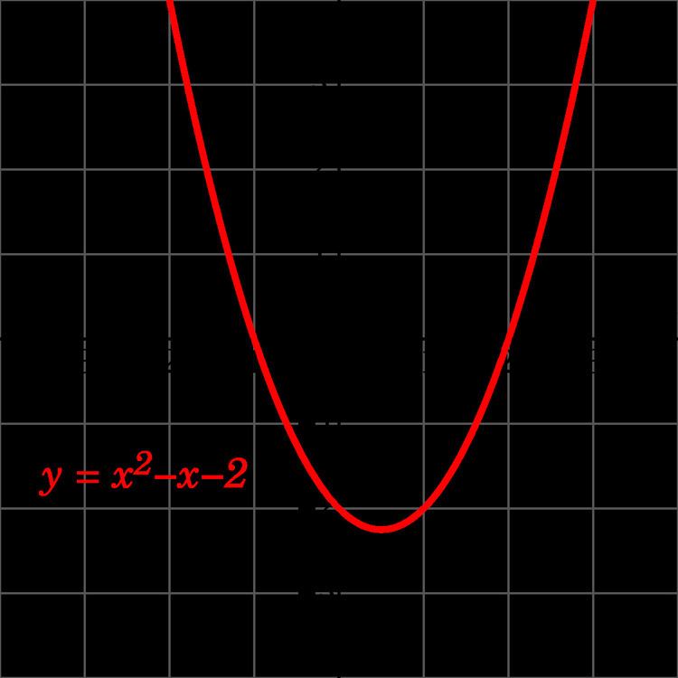
A quadratic equation is one which includes a term with an exponent of 2, for example, x 2 , and no term with higher exponent. The name derives from the Latin quadrus, meaning square. In general, a quadratic equation can be expressed in the form a x 2 + b x + c = 0 , where a is not zero (if it were zero, then the equation would not be quadratic but linear). Because of this a quadratic equation must contain the term a x 2 , which is known as the quadratic term. Hence a ≠ 0 , and so we may divide by a and rearrange the equation into the standard form

x 2 + p x + q = 0

where p = b / a and q = c / a . Solving this, by a process known as completing the square, leads to the quadratic formula

x = − b ± b 2 − 4 a c 2 a ,

where the symbol "±" indicates that both

x = − b + b 2 − 4 a c 2 a and x = − b − b 2 − 4 a c 2 a

are solutions of the quadratic equation.

Quadratic equations can also be solved using factorization (the reverse process of which is expansion, but for two linear terms is sometimes denoted foiling). As an example of factoring:

x 2 + 3 x − 10 = 0 ,

which is the same thing as

( x + 5 ) ( x − 2 ) = 0.

It follows from the zero-product property that either x = 2 or x = − 5 are the solutions, since precisely one of the factors must be equal to zero. All quadratic equations will have two solutions in the complex number system, but need not have any in the real number system. For example,

x 2 + 1 = 0

has no real number solution since no real number squared equals −1. Sometimes a quadratic equation has a root of multiplicity 2, such as:

( x + 1 ) 2 = 0.

For this equation, −1 is a root of multiplicity 2. This means −1 appears two times, since the equation can be rewritten in factored form as

[ x − ( − 1 ) ] [ x − ( − 1 ) ] = 0.

Complex numbers

All quadratic equations have two solutions in complex numbers, a category that includes real numbers, imaginary numbers, and sums of real and imaginary numbers. Complex numbers first arise in the teaching of quadratic equations and the quadratic formula. For example, the quadratic equation

x 2 + x + 1 = 0

has solutions

x = − 1 + − 3 2 and x = − 1 − − 3 2 .

Since − 3 is not any real number, both of these solutions for x are complex numbers.

Exponential and logarithmic equations

An exponential equation is one which has the form a x = b for a > 0 , which has solution

X = log a ⁡ b = ln ⁡ b ln ⁡ a

when b > 0 . Elementary algebraic techniques are used to rewrite a given equation in the above way before arriving at the solution. For example, if

3 ⋅ 2 x − 1 + 1 = 10

then, by subtracting 1 from both sides of the equation, and then dividing both sides by 3 we obtain

2 x − 1 = 3

whence

x − 1 = log 2 ⁡ 3

or

x = log 2 ⁡ 3 + 1.

A logarithmic equation is an equation of the form l o g a ( x ) = b for a > 0 , which has solution

X = a b .

For example, if

4 log 5 ⁡ ( x − 3 ) − 2 = 6

then, by adding 2 to both sides of the equation, followed by dividing both sides by 4, we get

log 5 ⁡ ( x − 3 ) = 2

whence

x − 3 = 5 2 = 25

from which we obtain

x = 28.

Radical equations

A radical equation is one that includes a radical sign, which includes square roots, x , cube roots, x 3 , and nth roots, x n . Recall that an nth root can be rewritten in exponential format, so that x n is equivalent to x 1 n . Combined with regular exponents (powers), then x 3 2 (the square root of x cubed), can be rewritten as x 3 2 . So a common form of a radical equation is x m n = a (equivalent to x m n = a ) where m and n are integers. It has real solution(s):

For example, if:

( x + 5 ) 2 / 3 = 4 ,

then

x + 5 = ± ( 4 ) 3 x + 5 = ± 8 x = − 5 ± 8 x = 3 , − 13 .

System of linear equations

There are different methods to solve a system of linear equations with two variables.

Elimination method

An example of solving a system of linear equations is by using the elimination method:

{ 4 x + 2 y = 14 2 x − y = 1.

Multiplying the terms in the second equation by 2:

4 x + 2 y = 14 4 x − 2 y = 2.

Adding the two equations together to get:

8 x = 16

which simplifies to

x = 2.

Since the fact that x = 2 is known, it is then possible to deduce that y = 3 by either of the original two equations (by using 2 instead of x ) The full solution to this problem is then

{ x = 2 y = 3.

Note that this is not the only way to solve this specific system; y could have been solved before x .

Substitution method

Another way of solving the same system of linear equations is by substitution.

{ 4 x + 2 y = 14 2 x − y = 1.

An equivalent for y can be deduced by using one of the two equations. Using the second equation:

2 x − y = 1

Subtracting 2 x from each side of the equation:

2 x − 2 x − y = 1 − 2 x − y = 1 − 2 x

and multiplying by −1:

y = 2 x − 1.

Using this y value in the first equation in the original system:

4 x + 2 ( 2 x − 1 ) = 14 4 x + 4 x − 2 = 14 8 x − 2 = 14

Adding 2 on each side of the equation:

8 x − 2 + 2 = 14 + 2 8 x = 16

which simplifies to

x = 2

Using this value in one of the equations, the same solution as in the previous method is obtained.

{ x = 2 y = 3.

Note that this is not the only way to solve this specific system; in this case as well, y could have been solved before x .

Inconsistent systems

In the above example, a solution exists. However, there are also systems of equations which do not have any solution. Such a system is called inconsistent. An obvious example is

{ x + y = 1 0 x + 0 y = 2 .

As 0≠2, the second equation in the system has no solution. Therefore, the system has no solution. However, not all inconsistent systems are recognized at first sight. As an example, let us consider the system

{ 4 x + 2 y = 12 − 2 x − y = − 4 .

Multiplying by 2 both sides of the second equation, and adding it to the first one results in

0 x + 0 y = 4 ,

which has clearly no solution.

Undetermined systems

There are also systems which have infinitely many solutions, in contrast to a system with a unique solution (meaning, a unique pair of values for x and y ) For example:

{ 4 x + 2 y = 12 − 2 x − y = − 6

Isolating y in the second equation:

y = − 2 x + 6

And using this value in the first equation in the system:

4 x + 2 ( − 2 x + 6 ) = 12 4 x − 4 x + 12 = 12 12 = 12

The equality is true, but it does not provide a value for x . Indeed, one can easily verify (by just filling in some values of x ) that for any x there is a solution as long as y = − 2 x + 6 . There is an infinite number of solutions for this system.

Over- and underdetermined systems

Systems with more variables than the number of linear equations are called underdetermined. Such a system, if it has any solutions, does not have a unique one but rather an infinitude of them. An example of such a system is

{ x + 2 y = 10 y − z = 2.

When trying to solve it, one is led to express some variables as functions of the other ones if any solutions exist, but cannot express all solutions numerically because there are an infinite number of them if there are any.

A system with a greater number of equations than variables is called overdetermined. If an overdetermined system has any solutions, necessarily some equations are linear combinations of the others.