Electronic filter topology

Passive topologies

Passive filters have been long in development and use. Most are built from simple two-port networks called "sections". There is no formal definition of a section except that it must have at least one series component and one shunt component. Sections are invariably connected in a "cascade" or "daisy-chain" topology, consisting of additional copies of the same section or of completely different sections. The rules of series and parallel impedance would combine two sections consisting only of series components or shunt components into a single section.

Some passive filters, consisting of only one or two filter sections, are given special names including the L-section, T-section and Π-section, which are unbalanced filters, and the C-section, H-section and box-section, which are balanced. All are built upon a very simple "ladder" topology (see below). The chart at the bottom of the page shows these various topologies in terms of general constant k filters.

Filters designed using network synthesis usually repeat the simplest form of L-section topology though component values may change in each section. Image designed filters, on the other hand, keep the same basic component values from section to section though the topology may vary and tend to make use of more complex sections.

L-sections are never symmetrical but two L-sections back-to-back form a symmetrical topology and many other sections are symmetrical in form.

Ladder topologies

Ladder topology, often called Cauer topology after Wilhelm Cauer (inventor of the elliptic filter), was in fact first used by George Campbell (inventor of the constant k filter). Campbell published in 1922 but had clearly been using the topology for some time before this. Cauer first picked up on ladders (published 1926) inspired by the work of Foster (1924). There are two forms of basic ladder topologies; unbalanced and balanced. Cauer topology is usually thought of as an unbalanced ladder topology.

A ladder network consists of cascaded asymmetrical L-sections (unbalanced) or C-sections (balanced). In low pass form the topology would consist of series inductors and shunt capacitors. Other bandforms would have an equally simple topology transformed from the lowpass topology. The transformed network will have shunt admittances that are dual networks of the series impedances if they were duals in the starting network - which is the case with series inductors and shunt capacitors.

Modified ladder topologies

Image filter design commonly uses modifications of the basic ladder topology. These topologies, invented by Otto Zobel, have the same passbands as the ladder on which they are based but their transfer functions are modified to improve some parameter such as impedance matching, stopband rejection or passband-to-stopband transition steepness. Usually the design applies some transform to a simple ladder topology: the resulting topology is ladder-like but no longer obeys the rule that shunt admittances are the dual network of series impedances: it invariably becomes more complex with higher component count. Such topologies include;

m-derived filter

mm'-type filter

General m_n-type filter

The m-type (m-derived) filter is by far the most commonly used modified image ladder topology. There are two m-type topologies for each of the basic ladder topologies; the series-derived and shunt-derived topologies. These have identical transfer functions to each other but different image impedances. Where a filter is being designed with more than one passband, the m-type topology will result in a filter where each passband has an analogous frequency-domain response. It is possible to generalise the m-type topology for filters with more than one passband using parameters m₁, m₂, m₃ etc., which are not equal to each other resulting in general m_n-type filters which have bandforms that can differ in different parts of the frequency spectrum.

The mm'-type topology can be thought of as a double m-type design. Like the m-type it has the same bandform but offers further improved transfer characteristics. It is, however, a rarely used design due to increased component count and complexity as well as its normally requiring basic ladder and m-type sections in the same filter for impedance matching reasons. It is normally only found in a composite filter.

Bridged-T topologies

Zobel constant resistance filters use a topology that is somewhat different from other filter types, distinguished by having a constant input resistance at all frequencies and in that they use resistive components in the design of their sections. The higher component and section count of these designs usually limits their use to equalisation applications. Topologies usually associated with constant resistance filters are the bridged-T and its variants, all described in the Zobel network article;

Bridged-T topology

Balanced bridged-T topology

Open-circuit L-section topology

Short-circuit L-section topology

Balanced open-circuit C-section topology

Balanced short-circuit C-section topology

The bridged-T topology is also used in sections intended to produce a signal delay but in this case no resistive components are used in the design.

Lattice topology

Both the T-section (from ladder topology) and the bridge-T (from Zobel topology) can be transformed into a lattice topology filter section but in both cases this results in high component count and complexity. The most common application of lattice filters (X-sections) is in all-pass filters used for phase equalisation.

Although T and bridged-T sections can always be transformed into X-sections the reverse is not always possible because of the possibility of negative values of inductance and capacitance arising in the transform.

Lattice topology is identical to the more familiar bridge topology, the difference being merely the drawn representation on the page rather than any real difference in topology, circuitry or function.

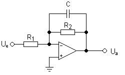
Multiple feedback topology

Multiple feedback topology is an electronic filter topology which is used to implement an electronic filter by adding two poles to the transfer function. A diagram of the circuit topology for a second order low pass filter is shown in the figure on the right.

The transfer function of the multiple feedback topology circuit, like all second-order linear filters, is:

H ( s ) = V o V i = − 1 A s 2 + B s + C = K ω 0 2 s 2 + ω 0 Q s + ω 0 2 .

In an MF filter,

A = ( R 1 R 3 C 2 C 5 ) B = R 3 C 5 + R 1 C 5 + R 1 R 3 C 5 / R 4 C = R 1 / R 4 Q = R 3 R 4 C 2 C 5 ( R 4 + R 3 + | K | R 3 ) C 5 is the Q factor. K = − R 4 / R 1 is the DC voltage gain ω 0 = 2 π f 0 = 1 / R 3 R 4 C 2 C 5 is the corner frequency

Biquad filter

For the digital implementation of a biquad filter, check Digital biquad filter.

A biquad filter is a type of linear filter that implements a transfer function that is the ratio of two quadratic functions. The name biquad is short for biquadratic. It is also sometimes called the 'ring of 3' circuit.

Biquad filters are typically active and implemented with a single-amplifier biquad (SAB) or two-integrator-loop topology.

The SAB topology uses feedback to generate complex poles and possibly complex zeros. In particular, the feedback moves the real poles of an RC circuit in order to generate the proper filter characteristics.

The two-integrator-loop topology is derived from rearranging a biquadratic transfer function. The rearrangement will equate one signal with the sum of another signal, its integral, and the integral's integral. In other words, the rearrangement reveals a state variable filter structure. By using different states as outputs, any kind of second-order filter can be implemented.

The SAB topology is sensitive to component choice and can be more difficult to adjust. Hence, usually the term biquad refers to the two-integrator-loop state variable filter topology.

Tow-Thomas Biquad Example

For example, the basic configuration in Figure 1 can be used as either a low-pass or bandpass filter depending on where the output signal is taken from.

The second-order low-pass transfer function is given by

H ( s ) = G l p f ω 0 2 s 2 + ω 0 Q s + ω 0 2

where low-pass gain G l p f = − R 2 / R 1 . The second-order bandpass transfer function is given by

H ( s ) = G b p f ω 0 Q s s 2 + ω 0 Q s + ω 0 2 .

with bandpass gain G b p f = − R 3 / R 1 . In both cases, the

Natural frequency is ω 0 = 1 / R 2 R 4 C 1 C 2 .

Quality factor is Q = R 3 2 C 1 R 2 R 4 C 2 .

The bandwidth is approximated by B = ω 0 / Q , and Q is sometimes expressed as a damping constant ζ = 1 / 2 Q . If a noninverting low-pass filter is required, the output can be taken at the output of the second operational amplifier, after the order of the second integrator and the inverter has been switched. If a noninverting bandpass filter is required, the order of the second integrator and the inverter can be switched, and the output taken at the output of the inverter's operational amplifier.