
 | ||
Prototype filters are electronic filter designs that are used as a template to produce a modified filter design for a particular application. They are an example of a nondimensionalised design from which the desired filter can be scaled or transformed. They are most often seen in regard to electronic filters and especially linear analogue passive filters. However, in principle, the method can be applied to any kind of linear filter or signal processing, including mechanical, acoustic and optical filters.
Contents
- Low pass prototype
- Frequency scaling
- Impedance scaling
- Bandform transformation
- Lowpass to highpass
- Lowpass to bandpass
- Lowpass to bandstop
- Lowpass to multi band
- Alternative prototype
- References
Filters are required to operate at many different frequencies, impedances and bandwidths. The utility of a prototype filter comes from the property that all these other filters can be derived from it by applying a scaling factor to the components of the prototype. The filter design need thus only be carried out once in full, with other filters being obtained by simply applying a scaling factor.
Especially useful is the ability to transform from one bandform to another. In this case, the transform is more than a simple scale factor. Bandform here is meant to indicate the category of passband that the filter possesses. The usual bandforms are lowpass, highpass, bandpass and bandstop, but others are possible. In particular, it is possible for a filter to have multiple passbands. In fact, in some treatments, the bandstop filter is considered to be a type of multiple passband filter having two passbands. Most commonly, the prototype filter is expressed as a lowpass filter, but other techniques are possible.
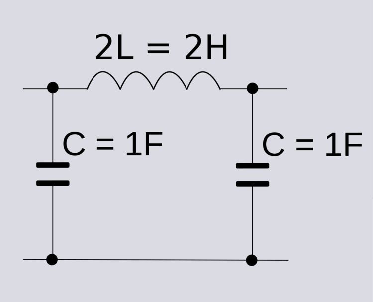
Parts of this article or section rely on the reader's knowledge of the complex impedance representation of capacitors and inductors and on knowledge of the frequency domain representation of signals.Low-pass prototype
The prototype is most often a low-pass filter with a 3 dB corner frequency of angular frequency ωc' = 1 rad/s. Occasionally, frequency f' ' = 1 Hz is used instead of ωc' = 1. Likewise, the nominal or characteristic impedance of the filter is set to R ' = 1 Ω.
In principle, any non-zero frequency point on the filter response could be used as a reference for the prototype design. For example, for filters with ripple in the passband, the corner frequency is usually defined as the highest frequency at maximum ripple rather than 3 dB. Another case is in image parameter filters (an older design method than the more modern network synthesis filters) which use the cut-off frequency rather than the 3 dB point since cut-off is a well-defined point in this type of filter.
The prototype filter can only be used to produce other filters of the same class and order. For instance, a fifth-order Bessel filter prototype can be converted into any other fifth-order Bessel filter, but it cannot be transformed into a third-order Bessel filter or a fifth-order Tchebyscheff filter.
Frequency scaling
The prototype filter is scaled to the frequency required with the following transformation:
where ωc' is the value of the frequency parameter (e.g. cut-off frequency) for the prototype and ωc is the desired value. So if ωc' = 1 then the transfer function of the filter is transformed as:
It can readily be seen that to achieve this, the non-resistive components of the filter must be transformed by:
Impedance scaling
Impedance scaling is invariably a scaling to a fixed resistance. This is because the terminations of the filter, at least nominally, are taken to be a fixed resistance. To carry out this scaling to a nominal impedance R, each impedance element of the filter is transformed by:
It may be more convenient on some elements to scale the admittance instead:
It can readily be seen that to achieve this, the non-resistive components of the filter must be scaled as:
Impedance scaling by itself has no effect on the transfer function of the filter (providing that the terminating impedances have the same scaling applied to them). However, it is usual to combine the frequency and impedance scaling into a single step:
Bandform transformation
In general, the bandform of a filter is transformed by replacing iω where it occurs in the transfer function with a function of iω. This in turn leads to the transformation of the impedance components of the filter into some other component(s). The frequency scaling above is a trivial case of bandform transformation corresponding to a lowpass to lowpass transformation.
Lowpass to highpass
The frequency transformation required in this case is:
where ωc is the point on the highpass filter corresponding to ωc' on the prototype. The transfer function then transforms as:
Inductors are transformed into capacitors according to,
and capacitors are transformed into inductors,
the primed quantities being the component value in the prototype.
Lowpass to bandpass
In this case, the required frequency transformation is:
where Q is the Q-factor and is equal to the inverse of the fractional bandwidth:
If ω1 and ω2 are the lower and upper frequency points (respectively) of the bandpass response corresponding to ωc' of the prototype, then,
Δω is the absolute bandwidth, and ω0 is the resonant frequency of the resonators in the filter. Note that frequency scaling the prototype prior to lowpass to bandpass transformation does not affect the resonant frequency, but instead affects the final bandwidth of the filter.
The transfer function of the filter is transformed according to:
Inductors are transformed into series resonators,
and capacitors are transformed into parallel resonators,
Lowpass to bandstop
The required frequency transformation for lowpass to bandstop is:
Inductors are transformed into parallel resonators,
and capacitors are transformed into series resonators,
Lowpass to multi-band
Filters with multiple passbands may be obtained by applying the general transformation:
The number of resonators in the expression corresponds to the number of passbands required. Lowpass and highpass filters can be viewed as special cases of the resonator expression with one or the other of the terms becoming zero as appropriate. Bandstop filters can be regarded as a combination of a lowpass and a highpass filter. Multiple bandstop filters can always be expressed in terms of a multiple bandpass filter. In this way it, can be seen that this transformation represents the general case for any bandform, and all the other transformations are to be viewed as special cases of it.
The same response can equivalently be obtained, sometimes with a more convenient component topology, by transforming to multiple stopbands instead of multiple passbands. The required transformation in those cases is:
Alternative prototype
In his treatment of image filters, Zobel provided an alternative basis for constructing a prototype which is not based in the frequency domain. The Zobel prototypes do not, therefore, correspond to any particular bandform, but they can be transformed into any of them. Not giving special significance to any one bandform makes the method more mathematically pleasing; however, it is not in common use.
The Zobel prototype considers filter sections, rather than components. That is, the transformation is carried out on a two-port network rather than a two-terminal inductor or capacitor. The transfer function is expressed in terms of the product of the series impedance, Z, and the shunt admittance Y of a filter half-section. See the article Image impedance for a description of half-sections. This quantity is nondimensional, adding to the prototype's generality. Generally, ZY is a complex quantity,
With image filters, it is possible to obtain filters of different classes from the constant k filter prototype by means of a different kind of transformation (see composite image filter), constant k being those filters for which Z/Y is a constant. For this reason, filters of all classes are given in terms of U(ω) for a constant k, which is notated as,
In the case of dissipationless networks, i.e. no resistors, the quantity V(ω) is zero and only U(ω) need be considered. Uk(ω) ranges from 0 at the centre of the passband to -1 at the cut-off frequency and then continues to increase negatively into the stopband regardless of the bandform of the filter being designed. To obtain the required bandform, the following transforms are used:
For a lowpass constant k prototype that is scaled:
the independent variable of the response plot is,
The bandform transformations from this prototype are,
for lowpass,
for highpass,
and for bandpass,