Dynamic substructuring

History

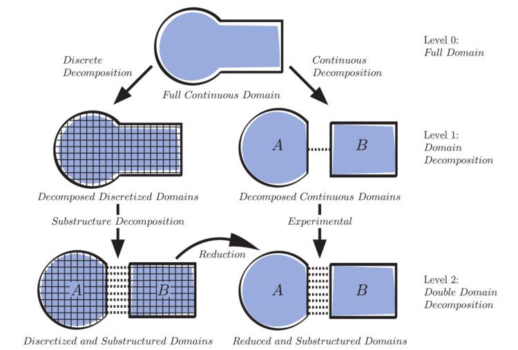
The roots of dynamic substructuring can be found in the field of domain decomposition. In 1890 the mathematician Hermann Schwarz came up with an iterative procedure for domain decomposition which allows to solve for continuous coupled subdomains. However, many of the analytical models of coupled continuous subdomains do not have closed-form solutions, which led to discretization and approximation techniques such as the Ritz method (which is sometimes called the Raleigh-Ritz method due the similarity between Ritz's formulation and the Raleigh ratio) the boundary element method (BEM) and the finite element method (FEM). These methods can be considered as "first level" domain decomposition techniques.

The finite element method proved to be the most efficient method and the invention of the microprocessor made it possible to easily solve a large variety of physical problems. In order to analyse even larger and more complex problems, methods were invented to optimize the efficiency of the discretized calculations. The first step was replacing the direct solvers by iterative solvers such as the conjugate gradient method. The lack of robustness and slow convergence of these solvers did not make them an interesting alternative in the beginning. The rise of parallel computing in the 1980s however sparked their popularity. Complex problems could now be solved by dividing the problem into subdomains, each processed by a separate processor, and solving for the interface coupling iteratively. This can be seen as a second level domain decomposition as is visualized in the figure.

The efficiency of dynamic modelling could be increased even further by reducing the complexity of the individual subdomains. This reduction of the subdomains (or substructures in the context of structural dynamics) is realized by representing substructures by means of their general responses. Expressing the separate substructures by means of their general response instead of their detailed discretization led to the so-called dynamic substructuring method. This reduction step also allowed for replacing the mathematical description of the domains by experimentally obtained information. This reduction step is also visualized by the reduction arrow in the figure.

The first dynamic substructuring methods were developed in the 1960s and were more commonly known under the name component mode synthesis (CMS). The benefits of dynamic substructuring were quickly discovered by the scientific and engineering communities and it became an important research topic in the field of structural dynamics and vibrations. Major developments followed, resulting in e.g. the classic Craig-Bampton method.

Due to improvements in sensor and signal processing technology in the 1980s, substructuring techniques also became attractive for the experimental community. Methods dealing with structural dynamic modification were created in which coupling techniques were directly applied to measured frequency response functions (FRFs). Broad popularity of the method was gained when Jetmundsen et al. formulated the classical frequency-based substructuring (FBS) method, which laid the ground work for frequency-based dynamic substructuring. In 2006 a systematic notation was introduced by De Klerk et al. in order to simplify the difficult and elaborate notation that had been used prior. The simplification was done by means of two Boolean matrices that handle all the "bookkeeping" involved in the assembly of substructures

Domains

Dynamic substructuring can best be seen as a domain-independent toolset for assembly of component models, rather than a modelling method of its own. Generally, dynamic substructuring can be used for all domains that are well suited to simulate multiple input/multiple output behaviour. Five domains that are well suited for substructuring are:

The physical domain concerns methods that are based on (linearised) mass, damping and stiffness matrices, typically obtained from numerical FEM modelling. Popular solutions to solve the associated system of second order differential equations are the time integration schemes of Newmark and the Hilbert-Hughes-Taylor scheme. The modal domain concerns component mode synthesis (CMS) techniques such as the Craig-Bampton, Rubin and McNeal method. These methods provide efficient modal reduction bases and assembly techniques for numerical models in the physical domain. The frequency domain is more popularly known as Frequency Based Substructuring (FBS). Based on the classic formulation of Jetmundsen et al. and the reformulation of De Klerk et al., it has become the most commonly used domain for substructuring, because of the ease of expressing the differential equations of a dynamical system (by means of Frequency Response Functions, FRFs) and the convenience of implementing experimentally obtained models. The time domain refers to the recently proposed concept of Impulse Based Substructuring (IBS), which expresses the behaviour of a dynamic system using a set of Impulse Response Functions (IRFs). The state-space domain, finally, refers to methods proposed by Sjövall et al. that employ system identification techniques common to control theory.

An overview of the governing equations of the five herementioned domains is presented in the table below.

As dynamic substructuring is a domain-independent toolset, it is applicable to the dynamic equations of all domains. In order to establish substructure assembly in a particular domain, two interface conditions need to be implemented. This is explained next, followed by a few common substructuring techniques.

Interface Conditions

To establish substructuring coupling / decoupling in each of the above-mentioned domains, two conditions should be met:

These are the two essential conditions that keep substructures together, hence allow to construct an assembly of multiple components. Note that the conditions are comparable with Kirchhoff's laws for electric circuits, in which case similar conditions apply to currents and voltages though/over electric components in a network; see also Mechanical-electrical analogies.

Substructure connectivity

Consider two substructures A and B as depicted in the figure. The two substructures comprise a total of six nodes; the displacements of the nodes are described by a set of Degrees of Freedom (DoFs). The DoFs of the six nodes are partitioned as follows:

1. DoFs of the internal nodes of substructure A;
2. DoFs of the coupling nodes of substructures A and B, i.e. interface DoFs;
3. DoFs of the internal nodes of substructure B.

Note that the denotation 1, 2 and 3 indicates the function of the nodes/DoFs rather than the total amount. Let us define the sets of DoFs for the two substructures A and B in concatenated form. The displacements and applied forces are represented by the sets u and f . For the purpose of substructuring, a set of interface forces g is introduced which only contains non-zero entries on the interface DoFs:

The relation between dynamic displacements u and applied forces f of the uncoupled problem is governed by a particular dynamic equation, such as presented in the table above. The uncoupled equations of motion are augmented by extra terms/equations for compatibility and equilibrium, as discussed next.

Compatibility

The compatibility condition requires that the interface DoFs have the same sign and value at both sides of the interface: u 2 A = u 2 B . This condition can be expressed using a so-called signed Boolean matrix, denoted by B . For the given example this can be expressed as:

In some cases the interface nodes of the substructures are non-conforming, e.g. when two substructures are meshed separately. In such cases a non-Boolean matrix B has to be used in order to enforce a weak interface compatibility.

A second form in which the compatibility condition can be expressed is by means of coordinate substitution by a set of generalised coordinates q . The set q contains the unique coordinates that remain after assembly of the substructures Every matching pair of interface DoFs is described by a single generalised coordinate, which means that the compatibility condition is automatically enforced. Expressing u using q gives:

Matrix L is referred to as the Boolean localisation matrix. A useful relation between matrix B and L can be exposed by noting that compatibility should hold for any set of physical coordinates u expressed by q . Indeed, substituting u = L q in the equation B u = 0 :

Hence L represents the nullspace of B :

This means in practice that one only needs to define B or L ; the other Boolean matrix is calculated using the nullspace property.

Equilibrium

The second condition that has to be satisfied for substructure assembly is the force equilibrium for matching interface forces g . For the current example, this condition can be written as g 2 A = − g 2 B . Similar to the compatibility equation, the force equilibrium condition can be expressed using a Boolean matrix. Use is made of the transpose of the Boolean localisation matrix L that was introduced to write compatibility:

The equations for g 1 and g 3 state that the interface forces on internal nodes are zero, hence not present. The equation for g 2 correctly establishes the force equilibrium between a matching pair of interface DoFs according to Newton's third law.

A second notation in which the equilibrium condition can be expressed is by introducing a set of Lagrange multipliers λ . The substitution of these Lagrange multipliers is possible as g 2 A and g 2 B differ only in sign, not in value. Using again the signed Boolean matrix B :

The set λ defines the intensity of the interface forces g 2 . Each Lagrange multiplier represents the magnitude of two matching interface forces in the assembly. By defining the interface forces g using Lagrange multipliers λ , force equilibrium is automatically satisfied. This can be seen by substituting g = − B T λ into the first equilibrium equation:

Again, the nullspace property of the Boolean matrices is used here, namely: L T B T = 0 .

The two conditions as presented above can be applied to establish coupling / decoupling in a myriad of domains and are thus independent of variables such as time, frequency, mode, etc. Some implementations of the interface conditions for the most common domains of substructuring are presented below.

Substructuring in the physical domain

The physical domain is the domain that has the most straightforward physical interpretation. For each discrete linearised dynamic system one is able to write an equilibrium between the externally applied forces and the internal forces originating from intrinsic inertia, viscous damping and elasticity. This relation is governed by one of the most elementary formulas in structural vibrations:

M , C , K represent the mass, damping and stiffness matrix of the system. These matrices are often obtained from finite element modelling (FEM), and are referred to as the numerical model of the structure. Furthermore, u represents the DoFs and f the force vector which are dependent on time ( t ) . This dependency is omitted in the following equations in order to improve readability.

Coupling in the physical domain

Coupling of n substructures in the physical domain first requires writing the uncoupled equations of motion of the n substructures in block diagonal form:

Next, two assembly approaches can be distinguished: primal and dual assembly.

Primal assembly

For primal assembly, a unique set of degrees of freedom q is defined in order to satisfy compatibility, u = L q . Furthermore, a second equation is added to enforce interface force equilibrium. This results in the following coupled dynamic equilibrium equations:

Pre-multiplying the first equation by L T and noting that L T g = 0 , the primal assembly reduces to:

The primally assembled system matrices can be used for a transient simulation by any standard time stepping algorithm. Note that the primal assembly technique is analogue to assembly of super-elements in finite element methods.

Dual assembly

In the dual assembly formulation the global set of DoFs is retained and an assembly is made by a priori satisfying the equilibrium condition g = − B T λ . Again, the Lagrange multipliers represent the interface forces connecting the DoFs at the interface. As these are unknowns, they are moved to the left-hand side of the equation. In order to satisfy compatibility, a second equation is added to the system, now operating on the displacements:

The dually assembled system can be written in matrix form as:

This dually assembled system can also be used in a transient simulation by means of a standard time stepping algorithm.

Substructuring in the frequency domain

In order to write out the equations for frequency based substructuring (FBS), the dynamic equilibrium first has to be put in the frequency domain. Starting with the dynamic equilibrium in the physical domain:

Taking the Fourier transform of this equation gives the dynamic equilibrium in the frequency domain:

Matrix Z ( ω ) is referred to as the dynamic stiffness matrix. This matrix consists of the complex-valued frequency-dependent functions that describe the force required to generate a unit harmonic displacement at a certain DoF. The inverse of the matrix Z ( ω ) is defined as Y ( ω ) ≜ ( Z ( ω ) ) − 1 and yields the more intuitive admittance notation:

The receptance matrix Y ( ω ) contains the frequency response functions (FRFs) of the structure which describe the displacement response to a unit input force. Other variants of the receptance matrix are the mobility and accelerance matrix, which respectively describe the velocity and acceleration response. The elements of the dynamic stiffness (or impedance in general) and receptance (or admittance in general) matrix are defined as follows:

Coupling in the frequency domain

In order to couple two substructures in the frequency domain, use is made of the admittance and impedance matrices of both substructures. Using the definition of substructures A and B as introduced previously, the following impedance and admittance matrices are defined (note that the frequency dependency ( ω ) is omitted from the terms to improve readability):

The two admittance and impedance matrices can be put in block diagonal form in order to align with the global set of DoFs u :

The off-diagonal zero terms show that at this point no coupling is present between the two substructures. In order to create this coupling, use can be made of the primal or dual assembly method. Both assembly methods make use of the dynamic equations as was defined before:

In these equations g is again used to define the set of interface forces, which are yet unknown.

Primal assembly

In order to obtain the primal system of equations, a unique set of coordinates q is defined: u = L q . By definition of an appropriate Boolean localisation matrix L , a unique set of DoFs remains for which the compatibility condition is satisfied a priori (compatibility condition). In order to satisfy the equilibrium condition a second equation is added to the equations of motion:

Pre-multiplying the first equation with L T yields the notation of the assembled equations of motion for the generalised coordinates q :

This result can be rewritten in admittance form as:

This last result gives access to the generalised responses as a result of the generalised applied forces f ~ , namely by inverting the primally assembled impedance matrix.

The primal assembly procedure is mainly of interest when one has access to the dynamics in impedance form, e.g. from finite element modelling. When one only has access to the dynamics in admittance notation, the dual formulation is a more suitable approach.

Dual assembly

A dually assembled system starts with the system written in the admittance notation. For a dually assembled system the force equilibrium condiition is satisfied a priori by substituting Lagrange multipliers λ for the interface forces: g = − B T λ . The compatibility condition is enforced by adding an additional equation:

Substituting the first line in the second and solving for λ gives:

The term B Y f represents the incompatibility caused by the uncoupled responses of the substructures to the applied forces f . By multiplying the incompatibility with the combined interface stiffness, i.e. ( B Y B T ) − 1 , the forces λ that keep the substructures together are determined. The coupled response is obtained by substituting the calculated λ back into the original equation:

This coupling method is referred to as the Lagrange-multiplier frequency-based substructuring (LM-FBS) method. The LM-FBS method allows for quick and easy assembling of an arbitrary number of substructures in a systematic fashion. Note that the result Y ~ is theoretically the same as was obtained above by application of primal assembly.

Decoupling in the frequency domain

In addition to coupling of substructures, one is also able to decouple substructures from assemblies. Using the plus sign as a substructure coupling operator, the coupling procedure could simply be described as AB = A + B. Using a similar notation, decoupling could be formulated as AB - B = A. Decoupling procedures are often required to remove substructures that were added for measurement purposes, e.g. to fix the structure. Similar to coupling, a primal and dual formulation exists for decoupling procedures.

Primal disassembly

As a result of the primal coupling, the impedance matrix of the assembled system can be written as follows:

Using this relation, the following trivial subtraction operation would suffice for the decoupling of the substructure B from assembly AB:

By placing the impedance of AB and B in block-diagonal form, with a minus sign for the impedance of B to account for the subtraction operation, the same equation that was used for primal coupling can now be used to perform the primal decoupling procedures.

with:

The primal disassembly can thus be understood as the assembly of structure AB with the negative impedance of substructure B. A limitation of the primal disassembly is that all DoF of the substructure that is to be decoupled have to be exactly represented in the assembled situation. For numerical decoupling situations this should not pose any problems, however for experimental cases this can be troublesome. A solution to this problem can be found in the dual disassembly.

Dual disassembly

Similar to the dual assembly, the dual disassembly approaches the decoupling problem using the admittance matrices. Decoupling in the dual domain means finding a force that ensures compatibility, yet acts in the opposite direction. This newly found force would then counteract the force that is applied to the assembly due to the dynamics of substructure B. Writing this out in equations of motion:

In order to write the dynamics of both systems in one equation, using the LM-FBS assembly notation, the following matrices are defined:

In order to enforce compatibility, a similar approach is used as for the assembly task. Defining a B -matrix to enforce compatibility:

Using this notation, the disassembly procedure can be performed using exactly the same equation as was used for the dual assembly:

This means that coupling and decoupling procedures using LM-FBS require identical steps, the only difference being the manner in which the global admittance matrix is defined. Indeed, the substructures to couple appear with a plus sign, whereas decoupled structures carry a minus sign:

More advanced decoupling techniques use the fact that internal points of substructure B appear in both the admittances of AB and B, hence can be used to enhance the decoupling process. Such techniques are described in.