Kalpana Kalpana (Editor)

Drucker–Prager yield criterion

Updated on
Edit
Like
Comment
Share on FacebookTweet on TwitterShare on LinkedInShare on Reddit
Drucker–Prager yield criterion

The Drucker–Prager yield criterion is a pressure-dependent model for determining whether a material has failed or undergone plastic yielding. The criterion was introduced to deal with the plastic deformation of soils. It and its many variants have been applied to rock, concrete, polymers, foams, and other pressure-dependent materials.

Contents

The Drucker–Prager yield criterion has the form

J 2 = A + B   I 1

where I 1 is the first invariant of the Cauchy stress and J 2 is the second invariant of the deviatoric part of the Cauchy stress. The constants A , B are determined from experiments.

In terms of the equivalent stress (or von Mises stress) and the hydrostatic (or mean) stress, the Drucker–Prager criterion can be expressed as

σ e = a + b   σ m

where σ e is the equivalent stress, σ m is the hydrostatic stress, and a , b are material constants. The Drucker–Prager yield criterion expressed in Haigh–Westergaard coordinates is

1 2 ρ 3   B ξ = A

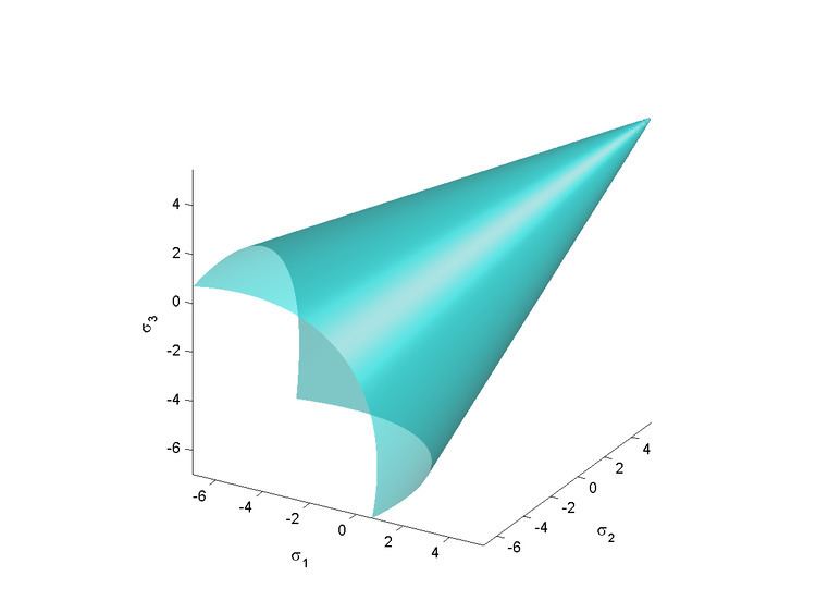
The Drucker–Prager yield surface is a smooth version of the Mohr–Coulomb yield surface.

Expressions for A and B

The Drucker–Prager model can be written in terms of the principal stresses as

1 6 [ ( σ 1 σ 2 ) 2 + ( σ 2 σ 3 ) 2 + ( σ 3 σ 1 ) 2 ] = A + B   ( σ 1 + σ 2 + σ 3 )   .

If σ t is the yield stress in uniaxial tension, the Drucker–Prager criterion implies

1 3   σ t = A + B   σ t   .

If σ c is the yield stress in uniaxial compression, the Drucker–Prager criterion implies

1 3   σ c = A B   σ c   .

Solving these two equations gives

A = 2 3   ( σ c   σ t σ c + σ t )   ;     B = 1 3   ( σ t σ c σ c + σ t )   .

Uniaxial asymmetry ratio

Different uniaxial yield stresses in tension and in compression are predicted by the Drucker–Prager model. The uniaxial asymmetry ratio for the Drucker–Prager model is

β = σ c σ t = 1 3   B 1 + 3   B   .

Expressions in terms of cohesion and friction angle

Since the Drucker–Prager yield surface is a smooth version of the Mohr–Coulomb yield surface, it is often expressed in terms of the cohesion ( c ) and the angle of internal friction ( ϕ ) that are used to describe the Mohr–Coulomb yield surface. If we assume that the Drucker–Prager yield surface circumscribes the Mohr–Coulomb yield surface then the expressions for A and B are

A = 6   c   cos ϕ 3 ( 3 sin ϕ )   ;     B = 2   sin ϕ 3 ( 3 sin ϕ )

If the Drucker–Prager yield surface middle circumscribes the Mohr–Coulomb yield surface then

A = 6   c   cos ϕ 3 ( 3 + sin ϕ )   ;     B = 2   sin ϕ 3 ( 3 + sin ϕ )

If the Drucker–Prager yield surface inscribes the Mohr–Coulomb yield surface then

A = 3   c   cos ϕ 9 + 3   sin 2 ϕ   ;     B = sin ϕ 9 + 3   sin 2 ϕ

Drucker–Prager model for polymers

The Drucker–Prager model has been used to model polymers such as polyoxymethylene and polypropylene. For polyoxymethylene the yield stress is a linear function of the pressure. However, polypropylene shows a quadratic pressure-dependence of the yield stress.

Drucker–Prager model for foams

For foams, the GAZT model uses

A = ± σ y 3   ;     B = 1 3   ( ρ 5   ρ s )

where σ y is a critical stress for failure in tension or compression, ρ is the density of the foam, and ρ s is the density of the base material.

Extensions of the isotropic Drucker–Prager model

The Drucker–Prager criterion can also be expressed in the alternative form

J 2 = ( A + B   I 1 ) 2 = a + b   I 1 + c   I 1 2   .

Deshpande–Fleck yield criterion or isotropic foam yield criterion

The Deshpande–Fleck yield criterion for foams has the form given in above equation. The parameters a , b , c for the Deshpande–Fleck criterion are

a = ( 1 + β 2 )   σ y 2   ,     b = 0   ,     c = β 2 3

where β is a parameter that determines the shape of the yield surface, and σ y is the yield stress in tension or compression.

Anisotropic Drucker–Prager yield criterion

An anisotropic form of the Drucker–Prager yield criterion is the Liu–Huang–Stout yield criterion. This yield criterion is an extension of the generalized Hill yield criterion and has the form

f := F ( σ 22 σ 33 ) 2 + G ( σ 33 σ 11 ) 2 + H ( σ 11 σ 22 ) 2 + 2 L σ 23 2 + 2 M σ 31 2 + 2 N σ 12 2 + I σ 11 + J σ 22 + K σ 33 1 0

The coefficients F , G , H , L , M , N , I , J , K are

F = 1 2 [ Σ 2 2 + Σ 3 2 Σ 1 2 ]   ;     G = 1 2 [ Σ 3 2 + Σ 1 2 Σ 2 2 ]   ;     H = 1 2 [ Σ 1 2 + Σ 2 2 Σ 3 2 ] L = 1 2 ( σ 23 y ) 2   ;     M = 1 2 ( σ 31 y ) 2   ;     N = 1 2 ( σ 12 y ) 2 I = σ 1 c σ 1 t 2 σ 1 c σ 1 t   ;     J = σ 2 c σ 2 t 2 σ 2 c σ 2 t   ;     K = σ 3 c σ 3 t 2 σ 3 c σ 3 t

where

Σ 1 := σ 1 c + σ 1 t 2 σ 1 c σ 1 t   ;     Σ 2 := σ 2 c + σ 2 t 2 σ 2 c σ 2 t   ;     Σ 3 := σ 3 c + σ 3 t 2 σ 3 c σ 3 t

and σ i c , i = 1 , 2 , 3 are the uniaxial yield stresses in compression in the three principal directions of anisotropy, σ i t , i = 1 , 2 , 3 are the uniaxial yield stresses in tension, and σ 23 y , σ 31 y , σ 12 y are the yield stresses in pure shear. It has been assumed in the above that the quantities σ 1 c , σ 2 c , σ 3 c are positive and σ 1 t , σ 2 t , σ 3 t are negative.

The Drucker yield criterion

The Drucker–Prager criterion should not be confused with the earlier Drucker criterion which is independent of the pressure ( I 1 ). The Drucker yield criterion has the form

f := J 2 3 α   J 3 2 k 2 0

where J 2 is the second invariant of the deviatoric stress, J 3 is the third invariant of the deviatoric stress, α is a constant that lies between -27/8 and 9/4 (for the yield surface to be convex), k is a constant that varies with the value of α . For α = 0 , k 2 = σ y 6 27 where σ y is the yield stress in uniaxial tension.

Anisotropic Drucker Criterion

An anisotropic version of the Drucker yield criterion is the Cazacu–Barlat (CZ) yield criterion which has the form

f := ( J 2 0 ) 3 α   ( J 3 0 ) 2 k 2 0

where J 2 0 , J 3 0 are generalized forms of the deviatoric stress and are defined as

J 2 0 := 1 6 [ a 1 ( σ 22 σ 33 ) 2 + a 2 ( σ 33 σ 11 ) 2 + a 3 ( σ 11 σ 22 ) 2 ] + a 4 σ 23 2 + a 5 σ 31 2 + a 6 σ 12 2 J 3 0 := 1 27 [ ( b 1 + b 2 ) σ 11 3 + ( b 3 + b 4 ) σ 22 3 + { 2 ( b 1 + b 4 ) ( b 2 + b 3 ) } σ 33 3 ] 1 9 [ ( b 1 σ 22 + b 2 σ 33 ) σ 11 2 + ( b 3 σ 33 + b 4 σ 11 ) σ 22 2 + { ( b 1 b 2 + b 4 ) σ 11 + ( b 1 b 3 + b 4 ) σ 22 } σ 33 2 ] + 2 9 ( b 1 + b 4 ) σ 11 σ 22 σ 33 + 2 b 11 σ 12 σ 23 σ 31 1 3 [ { 2 b 9 σ 22 b 8 σ 33 ( 2 b 9 b 8 ) σ 11 } σ 31 2 + { 2 b 10 σ 33 b 5 σ 22 ( 2 b 10 b 5 ) σ 11 } σ 12 2 { ( b 6 + b 7 ) σ 11 b 6 σ 22 b 7 σ 33 } σ 23 2 ]

Cazacu–Barlat yield criterion for plane stress

For thin sheet metals, the state of stress can be approximated as plane stress. In that case the Cazacu–Barlat yield criterion reduces to its two-dimensional version with

J 2 0 = 1 6 [ ( a 2 + a 3 ) σ 11 2 + ( a 1 + a 3 ) σ 22 2 2 a 3 σ 1 σ 2 ] + a 6 σ 12 2 J 3 0 = 1 27 [ ( b 1 + b 2 ) σ 11 3 + ( b 3 + b 4 ) σ 22 3 ] 1 9 [ b 1 σ 11 + b 4 σ 22 ] σ 11 σ 22 + 1 3 [ b 5 σ 22 + ( 2 b 10 b 5 ) σ 11 ] σ 12 2

For thin sheets of metals and alloys, the parameters of the Cazacu–Barlat yield criterion are

References

Drucker–Prager yield criterion Wikipedia