Complex quadratic polynomial - Alchetron, the free social encyclopedia

A complex quadratic polynomial is a quadratic polynomial whose coefficients and variable are complex numbers.

Forms

When the quadratic polynomial has only one variable (univariate), one can distinguish its 4 main forms:

The general form: f ( x ) = a 2 x 2 + a 1 x + a 0 where a 2 ≠ 0

The factored form used for logistic map f r ( x ) = r x ( 1 − x )

f θ ( x ) = x 2 + e 2 π θ i x which has an indifferent fixed point with multiplier λ = e 2 π θ i at the origin

The monic and centered form, f c ( x ) = x 2 + c

The monic and centered form has the following properties:

It is the simplest form of a nonlinear function with one coefficient (parameter),

It is an unicritical polynomial, i.e. it has one critical point,

It is a centered polynomial (the sum of its critical points is zero),

It can be postcritically finite, i.e. If the orbit of the critical point is finite. It is when critical point is periodic or preperiodic.

It is a unimodal function,

It is a rational function,

It is an entire function.

Between forms

Since f c ( x ) is affine conjugate to the general form of the quadratic polynomial it is often used to study complex dynamics and to create images of Mandelbrot, Julia and Fatou sets.

When one wants change from θ to c :

c = c ( θ ) = e 2 π θ i 2 ( 1 − e 2 π θ i 2 ) .

When one wants change from r to c , the parameter transformation is

c = c ( r ) = 1 − ( r − 1 ) 2 4 = − r 2 ( r − 2 2 )

and the transformation between the variables in z t + 1 = z t 2 + c and x t + 1 = r x t ( 1 − x t ) is

z = r ( 1 2 − x ) .

With doubling map

There is semi-conjugacy between the dyadic transformation (the doubling map) and the quadratic polynomial case of c = –2.

Map

The monic and centered form, sometimes called the Douady-Hubbard family of quadratic polynomials, is typically used with variable z and parameter c :

f c ( z ) = z 2 + c .

When it is used as an evolution function of the discrete nonlinear dynamical system

z n + 1 = f c ( z n )

it is named the quadratic map:

f c : z → z 2 + c .

The Mandelbrot set is the set of values of the parameter c for which the initial condition z₀ = 0 does not cause the iterates to diverge to infinity.

Notation

Here f n denotes the n-th iteration of the function f (and not exponentiation of the function):

f c n ( z ) = f c 1 ( f c n − 1 ( z ) )

so

z n = f c n ( z 0 ) .

Because of the possible confusion with exponentiation, some authors write f ∘ n for the nth iterate of the function f .

Critical point

A critical point of f c is a point z c r in the dynamical plane such that the derivative vanishes:

f c ′ ( z c r ) = 0.

Since

f c ′ ( z ) = d d z f c ( z ) = 2 z

implies

z c r = 0

we see that the only (finite) critical point of f c is the point z c r = 0 .

z 0 is an initial point for Mandelbrot set iteration.

Critical value

A critical value z c v of f c is the image of a critical point:

z c v = f c ( z c r )

Since

z c r = 0

we have

z c v = c .

So the parameter c is the critical value of f c ( z ) .

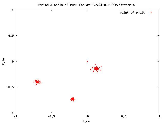
Critical orbit

The forward orbit of a critical point is called a critical orbit. Critical orbits are very important because every attracting periodic orbit attracts a critical point, so studying the critical orbits helps us understand the dynamics in the Fatou set.

z 0 = z c r = 0 z 1 = f c ( z 0 ) = c z 2 = f c ( z 1 ) = c 2 + c z 3 = f c ( z 2 ) = ( c 2 + c ) 2 + c . . .

This orbit falls into an attracting periodic cycle if one exists.

Critical sector

The critical sector is a sector of the dynamical plane containing the critical point.

Critical polynomial

P n ( c ) = f c n ( z c r ) = f c n ( 0 )

so

P 0 ( c ) = 0 P 1 ( c ) = c P 2 ( c ) = c 2 + c P 3 ( c ) = ( c 2 + c ) 2 + c

These polynomials are used for:

finding centers of these Mandelbrot set components of period n. Centers are roots of n-th critical polynomials

c e n t e r s = { c : P n ( c ) = 0 }

finding roots of Mandelbrot set components of period n (local minimum of P n ( c ) )

Misiurewicz points

M n , k = { c : P k ( c ) = P k + n ( c ) }

Critical curves

Diagrams of critical polynomials are called critical curves.

These curves create the skeleton (the dark lines) of a bifurcation diagram.

Planes

One can use the Julia-Mandelbrot 4-dimensional space for a global analysis of this dynamical system.

In this space there are 2 basic types of 2-D planes:

the dynamical (dynamic) plane, f c -plane or c-plane

the parameter plane or z-plane

There is also another plane used to analyze such dynamical systems w-plane:

the conjugation plane

model plane

Parameter plane

The phase space of a quadratic map is called its parameter plane. Here:

z 0 = z c r is constant and c is variable.

There is no dynamics here. It is only a set of parameter values. There are no orbits on the parameter plane.

The parameter plane consists of:

The Mandelbrot set

The bifurcation locus = boundary of Mandelbrot set

Bounded hyperbolic components of the Mandelbrot set = interior of Mandelbrot set

There are many different subtypes of the parameter plane.

Dynamical plane

On the dynamical plane one can find:

The Julia set

The Filled Julia set

The Fatou set

Orbits

The dynamical plane consists of:

Fatou set

Julia set

Here, c is a constant and z is a variable.

The two-dimensional dynamical plane can be treated as a Poincaré cross-section of three-dimensional space of continuous dynamical system.

Dynamical z-planes can be divided in two groups :

f 0 plane for c = 0 ( see complex squaring map )

f c planes ( all other planes for c ≠ 0 )

Derivative with respect to c

On the parameter plane:

c is a variable

z 0 = 0 is constant

The first derivative of f c n ( z 0 ) with respect to c is

z n ′ = d d c f c n ( z 0 ) .

This derivative can be found by iteration starting with

z 0 ′ = d d c f c 0 ( z 0 ) = 1

and then replacing at every consecutive step

z n + 1 ′ = d d c f c n + 1 ( z 0 ) = 2 ⋅ f c n ( z ) ⋅ d d c f c n ( z 0 ) + 1 = 2 ⋅ z n ⋅ z n ′ + 1.

This can easily be verified by using the chain rule for the derivative.

This derivative is used in the distance estimation method for drawing a Mandelbrot set.

Derivative with respect to z

On the dynamical plane:

z is a variable;

c is a constant.

At a fixed point z 0 ,

f c ′ ( z 0 ) = d d z f c ( z 0 ) = 2 z 0 .

At a periodic point z₀ of period p the first derivative of a function

( f c p ) ′ ( z 0 ) = d d z f c p ( z 0 ) = ∏ i = 0 p − 1 f c ′ ( z i ) = 2 p ∏ i = 0 p − 1 z i = λ

is often represented by λ and referred to as the multiplier or the Lyapunov characteristic number. It's logarithm is known as the Lyapunov exponent. It used to check the stability of periodic (also fixed) points.

At a nonperiodic point, the derivative, denoted by z n ′ , can be found by iteration starting with

z 0 ′ = 1 ,

and then using

z n ′ = 2 ∗ z n − 1 ∗ z n − 1 ′ .

This derivative is used for computing the external distance to the Julia set.

Schwarzian derivative

The Schwarzian derivative (SD for short) of f is:

( S f ) ( z ) = f ‴ ( z ) f ′ ( z ) − 3 2 ( f ″ ( z ) f ′ ( z ) ) 2 .

References

Complex quadratic polynomial Wikipedia

(Text) CC BY-SA

Contents