Neha Patil (Editor)

CMA ES

Updated on
Edit
Like
Comment
Share on FacebookTweet on TwitterShare on LinkedInShare on Reddit
CMA-ES

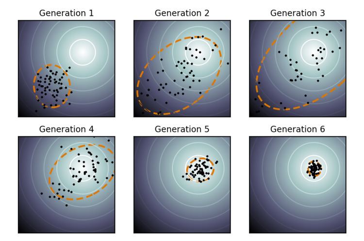
CMA-ES stands for Covariance Matrix Adaptation Evolution Strategy. Evolution strategies (ES) are stochastic, derivative-free methods for numerical optimization of non-linear or non-convex continuous optimization problems. They belong to the class of evolutionary algorithms and evolutionary computation. An evolutionary algorithm is broadly based on the principle of biological evolution, namely the repeated interplay of variation (via recombination and mutation) and selection: in each generation (iteration) new individuals (candidate solutions, denoted as x ) are generated by variation, usually in a stochastic way, of the current parental individuals. Then, some individuals are selected to become the parents in the next generation based on their fitness or objective function value f ( x ) . Like this, over the generation sequence, individuals with better and better f -values are generated.

Contents

In an evolution strategy, new candidate solutions are sampled according to a multivariate normal distribution in the R n . Recombination amounts to selecting a new mean value for the distribution. Mutation amounts to adding a random vector, a perturbation with zero mean. Pairwise dependencies between the variables in the distribution are represented by a covariance matrix. The covariance matrix adaptation (CMA) is a method to update the covariance matrix of this distribution. This is particularly useful, if the function f is ill-conditioned.

Adaptation of the covariance matrix amounts to learning a second order model of the underlying objective function similar to the approximation of the inverse Hessian matrix in the Quasi-Newton method in classical optimization. In contrast to most classical methods, fewer assumptions on the nature of the underlying objective function are made. Only the ranking between candidate solutions is exploited for learning the sample distribution and neither derivatives nor even the function values themselves are required by the method.

Principles

Two main principles for the adaptation of parameters of the search distribution are exploited in the CMA-ES algorithm.

First, a maximum-likelihood principle, based on the idea to increase the probability of successful candidate solutions and search steps. The mean of the distribution is updated such that the likelihood of previously successful candidate solutions is maximized. The covariance matrix of the distribution is updated (incrementally) such that the likelihood of previously successful search steps is increased. Both updates can be interpreted as a natural gradient descent. Also, in consequence, the CMA conducts an iterated principal components analysis of successful search steps while retaining all principal axes. Estimation of distribution algorithms and the Cross-Entropy Method are based on very similar ideas, but estimate (non-incrementally) the covariance matrix by maximizing the likelihood of successful solution points instead of successful search steps.

Second, two paths of the time evolution of the distribution mean of the strategy are recorded, called search or evolution paths. These paths contain significant information about the correlation between consecutive steps. Specifically, if consecutive steps are taken in a similar direction, the evolution paths become long. The evolution paths are exploited in two ways. One path is used for the covariance matrix adaptation procedure in place of single successful search steps and facilitates a possibly much faster variance increase of favorable directions. The other path is used to conduct an additional step-size control. This step-size control aims to make consecutive movements of the distribution mean orthogonal in expectation. The step-size control effectively prevents premature convergence yet allowing fast convergence to an optimum.

Algorithm

In the following the most commonly used (μ/μw, λ)-CMA-ES is outlined, where in each iteration step a weighted combination of the μ best out of λ new candidate solutions is used to update the distribution parameters. The main loop consists of three main parts: 1) sampling of new solutions, 2) re-ordering of the sampled solutions based on their fitness, 3) update of the internal state variables based on the re-ordered samples. A pseudocode of the algorithm looks as follows.

set λ // number of samples per iteration, at least two, generally > 4 initialize m , σ , C = I , p σ = 0 , p c = 0 // initialize state variables while not terminate // iterate for i in { 1... λ } // sample λ new solutions and evaluate them x i = sample_multivariate_normal(mean= m , covariance_matrix= σ 2 C ) f i = fitness( x i ) x 1... λ x s ( 1 ) . . . s ( λ ) with s ( i ) = argsort( f 1... λ , i ) // sort solutions m = m // we need later m m and x i m m ← update_m ( x 1 , . . . , x λ ) // move mean to better solutions p σ ← update_ps ( p σ , σ 1 C 1 / 2 ( m m ) ) // update isotropic evolution path p c ← update_pc ( p c , σ 1 ( m m ) , | | p σ | | ) // update anisotropic evolution path C ← update_C ( C , p c , ( x 1 m ) / σ , . . . , ( x λ m ) / σ ) // update covariance matrix σ ← update_sigma ( σ , | | p σ | | ) // update step-size using isotropic path length return m or x 1

The order of the five update assignments is relevant. In the following, the update equations for the five state variables are specified.

Given are the search space dimension n and the iteration step k . The five state variables are

m k R n , the distribution mean and current favorite solution to the optimization problem, σ k > 0 , the step-size, C k , a symmetric and positive definite n × n covariance matrix with C 0 = I and p σ R n , p c R n , two evolution paths, initially set to the zero vector.

The iteration starts with sampling λ > 1 candidate solutions x i R n from a multivariate normal distribution N ( m k , σ k 2 C k ) , i.e. for i = 1 , . . . , λ

The second line suggests the interpretation as perturbation (mutation) of the current favorite solution vector m k (the distribution mean vector). The candidate solutions x i are evaluated on the objective function f : R n R to be minimized. Denoting the f -sorted candidate solutions as

{ x i : λ | i = 1 λ } = { x i | i = 1 λ } and f ( x 1 : λ ) f ( x μ : λ ) f ( x μ + 1 : λ ) ,

the new mean value is computed as

where the positive (recombination) weights w 1 w 2 w μ > 0 sum to one. Typically, μ λ / 2 and the weights are chosen such that μ w := 1 / i = 1 μ w i 2 λ / 4 . The only feedback used from the objective function here and in the following is an ordering of the sampled candidate solutions due to the indices i : λ .

The step-size σ k is updated using cumulative step-size adaptation (CSA), sometimes also denoted as path length control. The evolution path (or search path) p σ is updated first.

where

c σ 1 n / 3 is the backward time horizon for the evolution path p σ and larger than one, μ w = ( i = 1 μ w i 2 ) 1 is the variance effective selection mass and 1 μ w μ by definition of w i , C k 1 / 2 = C k 1 = C k 1 is the unique symmetric square root of the inverse of C k , and d σ is the damping parameter usually close to one. For d σ = or c σ = 0 the step-size remains unchanged.

The step-size σ k is increased if and only if p σ is larger than the expected value

E N ( 0 , I ) = 2 Γ ( ( n + 1 ) / 2 ) / Γ ( n / 2 ) n ( 1 1 / ( 4 n ) + 1 / ( 21 n 2 ) )

and decreased if it is smaller. For this reason, the step-size update tends to make consecutive steps C k 1 -conjugate, in that after the adaptation has been successful ( m k + 2 m k + 1 σ k + 1 ) T C k 1 m k + 1 m k σ k 0 .

Finally, the covariance matrix is updated, where again the respective evolution path is updated first.

where T denotes the transpose and

c c 1 n / 4 is the backward time horizon for the evolution path p c and larger than one, α 1.5 and the indicator function 1 [ 0 , α n ] ( p σ ) evaluates to one iff p σ [ 0 , α n ] or, in other words, p σ α n , which is usually the case, c s = ( 1 1 [ 0 , α n ] ( p σ ) 2 ) c 1 c c ( 2 c c ) makes partly up for the small variance loss in case the indicator is zero, c 1 2 / n 2 is the learning rate for the rank-one update of the covariance matrix and c μ μ w / n 2 is the learning rate for the rank- μ update of the covariance matrix and must not exceed 1 c 1 .

The covariance matrix update tends to increase the likelihood for p c and for ( x i : λ m k ) / σ k to be sampled from N ( 0 , C k + 1 ) . This completes the iteration step.

The number of candidate samples per iteration, λ , is not determined a priori and can vary in a wide range. Smaller values, for example λ = 10 , lead to more local search behavior. Larger values, for example λ = 10 n with default value μ w λ / 4 , render the search more global. Sometimes the algorithm is repeatedly restarted with increasing λ by a factor of two for each restart. Besides of setting λ (or possibly μ instead, if for example λ is predetermined by the number of available processors), the above introduced parameters are not specific to the given objective function and therefore not meant to be modified by the user.

Theoretical foundations

Given the distribution parameters—mean, variances and covariances—the normal probability distribution for sampling new candidate solutions is the maximum entropy probability distribution over R n , that is, the sample distribution with the minimal amount of prior information built into the distribution. More considerations on the update equations of CMA-ES are made in the following.

Variable metric

The CMA-ES implements a stochastic variable-metric method. In the very particular case of a convex-quadratic objective function

the covariance matrix C k adapts to the inverse of the Hessian matrix H , up to a scalar factor and small random fluctuations. More general, also on the function g f , where g is strictly increasing and therefore order preserving and f is convex-quadratic, the covariance matrix C k adapts to H 1 , up to a scalar factor and small random fluctuations.

Maximum-likelihood updates

The update equations for mean and covariance matrix maximize a likelihood while resembling an expectation-maximization algorithm. The update of the mean vector m maximizes a log-likelihood, such that

where

denotes the log-likelihood of x from a multivariate normal distribution with mean m and any positive definite covariance matrix C . To see that m k + 1 is independent of C remark first that this is the case for any diagonal matrix C , because the coordinate-wise maximizer is independent of a scaling factor. Then, rotation of the data points or choosing C non-diagonal are equivalent.

The rank- μ update of the covariance matrix, that is, the right most summand in the update equation of C k , maximizes a log-likelihood in that

for μ n (otherwise C is singular, but substantially the same result holds for μ < n ). Here, p N ( x | C ) denotes the likelihood of x from a multivariate normal distribution with zero mean and covariance matrix C . Therefore, for c 1 = 0 and c μ = 1 , C k + 1 is the above maximum-likelihood estimator. See estimation of covariance matrices for details on the derivation.

Natural gradient descent in the space of sample distributions

Akimoto et al. and Glasmachers et al. discovered independently that the update of the distribution parameters resembles the descend in direction of a sampled natural gradient of the expected objective function value E f (x) (to be minimized), where the expectation is taken under the sample distribution. With the parameter setting of c σ = 0 and c 1 = 0 , i.e. without step-size control and rank-one update, CMA-ES can thus be viewed as an instantiation of Natural Evolution Strategies (NES). The natural gradient is independent of the parameterization of the distribution. Taken with respect to the parameters θ of the sample distribution p, the gradient of E f (x) can be expressed as

where p ( x ) = p ( x | θ ) depends on the parameter vector θ , the so-called score function, θ ln p ( x | θ ) = θ p ( x ) p ( x ) , indicates the relative sensitivity of p w.r.t. θ, and the expectation is taken with respect to the distribution p. The natural gradient of E f (x), complying with the Fisher information metric (an informational distance measure between probability distributions and the curvature of the relative entropy), now reads

where the Fisher information matrix F θ is the expectation of the Hessian of -lnp and renders the expression independent of the chosen parameterization. Combining the previous equalities we get

A Monte Carlo approximation of the latter expectation takes the average over λ samples from p

where the notation i : λ from above is used and therefore w i are monotonously decreasing in i .

Ollivier et al. finally found a rigorous derivation for the more robust weights, w i , as they are defined in the CMA-ES (weights are often zero for i > μ). They are formulated as the consistent estimator for the CDF of f ( X ) , X p ( . | θ ) at the point f ( x i : λ ) , composed with a fixed monotonous decreased transformation w , i.e.,

Let

such that p ( . | θ ) is the density of the multivariate normal distribution N ( m k , σ k 2 C k ) . Then, we have an explicit expression for the inverse of the Fisher information matrix where σ k is fixed

and for

and, after some calculations, the updates in the CMA-ES turn out as

m k + 1 = m k [ ~ E ^ θ ( f ) ] 1 , , n natural gradient for mean = m k + i = 1 λ w i ( x i : λ m k )

and

C k + 1 = C k + c 1 ( p c p c T C k ) c μ m a t ( [ ~ E ^ θ ( f ) ] n + 1 , , n + n 2 natural gradient for covariance matrix ) = C k + c 1 ( p c p c T C k ) + c μ i = 1 λ w i ( x i : λ m k σ k ( x i : λ m k σ k ) T C k )

where mat forms the proper matrix from the respective natural gradient sub-vector. That means, setting c 1 = c σ = 0 , the CMA-ES updates descend in direction of the approximation ~ E ^ θ ( f ) of the natural gradient while using different step-sizes (learning rates 1 and c μ ) for the orthogonal parameters m and C respectively. The most recent version of CMA-ES also use a different function w for m and C with negative values only for the latter (so-called active CMA).

Stationarity or unbiasedness

It is comparatively easy to see that the update equations of CMA-ES satisfy some stationarity conditions, in that they are essentially unbiased. Under neutral selection, where x i : λ N ( m k , σ k 2 C k ) , we find that

and under some mild additional assumptions on the initial conditions

and with an additional minor correction in the covariance matrix update for the case where the indicator function evaluates to zero, we find

Invariance

Invariance properties imply uniform performance on a class of objective functions. They have been argued to be an advantage, because they allow to generalize and predict the behavior of the algorithm and therefore strengthen the meaning of empirical results obtained on single functions. The following invariance properties have been established for CMA-ES.

  • Invariance under order-preserving transformations of the objective function value f , in that for any h : R n R the behavior is identical on f : x g ( h ( x ) ) for all strictly increasing g : R R . This invariance is easy to verify, because only the f -ranking is used in the algorithm, which is invariant under the choice of g .
  • Scale-invariance, in that for any h : R n R the behavior is independent of α > 0 for the objective function f : x h ( α x ) given σ 0 1 / α and m 0 1 / α .
  • Invariance under rotation of the search space in that for any h : R n R and any z R n the behavior on f : x h ( R x ) is independent of the orthogonal matrix R , given m 0 = R 1 z . More general, the algorithm is also invariant under general linear transformations R when additionally the initial covariance matrix is chosen as R 1 R 1 T .
  • Any serious parameter optimization method should be translation invariant, but most methods do not exhibit all the above described invariance properties. A prominent example with the same invariance properties is the Nelder–Mead method, where the initial simplex must be chosen respectively.

    Convergence

    Conceptual considerations like the scale-invariance property of the algorithm, the analysis of simpler evolution strategies, and overwhelming empirical evidence suggest that the algorithm converges on a large class of functions fast to the global optimum, denoted as x . On some functions, convergence occurs independently of the initial conditions with probability one. On some functions the probability is smaller than one and typically depends on the initial m 0 and σ 0 . Empirically, the fastest possible convergence rate in k for rank-based direct search methods can often be observed (depending on the context denoted as linear or log-linear or exponential convergence). Informally, we can write

    for some c > 0 , and more rigorously

    or similarly,

    This means that on average the distance to the optimum decreases in each iteration by a "constant" factor, namely by exp ( c ) . The convergence rate c is roughly 0.1 λ / n , given λ is not much larger than the dimension n . Even with optimal σ and C , the convergence rate c cannot largely exceed 0.25 λ / n , given the above recombination weights w i are all non-negative. The actual linear dependencies in λ and n are remarkable and they are in both cases the best one can hope for in this kind of algorithm. Yet, a rigorous proof of convergence is missing.

    Interpretation as coordinate-system transformation

    Using a non-identity covariance matrix for the multivariate normal distribution in evolution strategies is equivalent to a coordinate system transformation of the solution vectors, mainly because the sampling equation

    x i   m k + σ k × N ( 0 , C k )   m k + σ k × C k 1 / 2 N ( 0 , I )

    can be equivalently expressed in an "encoded space" as

    C k 1 / 2 x i represented in the encode space   C k 1 / 2 m k + σ k × N ( 0 , I )

    The covariance matrix defines a bijective transformation (encoding) for all solution vectors into a space, where the sampling takes place with identity covariance matrix. Because the update equations in the CMA-ES are invariant under linear coordinate system transformations, the CMA-ES can be re-written as an adaptive encoding procedure applied to a simple evolution strategy with identity covariance matrix. This adaptive encoding procedure is not confined to algorithms that sample from a multivariate normal distribution (like evolution strategies), but can in principle be applied to any iterative search method.

    Performance in practice

    In contrast to most other evolutionary algorithms, the CMA-ES is, from the users perspective, quasi parameter-free. The user has to choose an initial solution point, m 0 R n , and the initial step-size, σ 0 > 0 . Optionally, the number of candidate samples λ (population size) can be modified by the user in order to change the characteristic search behavior (see above) and termination conditions can or should be adjusted to the problem at hand.

    The CMA-ES has been empirically successful in hundreds of applications and is considered to be useful in particular on non-convex, non-separable, ill-conditioned, multi-modal or noisy objective functions. The search space dimension ranges typically between two and a few hundred. Assuming a black-box optimization scenario, where gradients are not available (or not useful) and function evaluations are the only considered cost of search, the CMA-ES method is likely to be outperformed by other methods in the following conditions:

  • on low-dimensional functions, say n < 5 , for example by the downhill simplex method or surrogate-based methods (like kriging with expected improvement);
  • on separable functions without or with only negligible dependencies between the design variables in particular in the case of multi-modality or large dimension, for example by differential evolution;
  • on (nearly) convex-quadratic functions with low or moderate condition number of the Hessian matrix, where BFGS or NEWUOA are typically ten times faster;
  • on functions that can already be solved with a comparatively small number of function evaluations, say no more than 10 n , where CMA-ES is often slower than, for example, NEWUOA or Multilevel Coordinate Search (MCS).
  • On separable functions, the performance disadvantage is likely to be most significant in that CMA-ES might not be able to find at all comparable solutions. On the other hand, on non-separable functions that are ill-conditioned or rugged or can only be solved with more than 100 n function evaluations, the CMA-ES shows most often superior performance.

    Variations and extensions

    The (1+1)-CMA-ES generates only one candidate solution per iteration step which becomes the new distribution mean if it is better than the current mean. For c c = 1 the (1+1)-CMA-ES is a close variant of Gaussian adaptation. Some Natural Evolution Strategies are close variants of the CMA-ES with specific parameter settings. Natural Evolution Strategies do not utilize evolution paths (that means in CMA-ES setting c c = c σ = 1 ) and they formalize the update of variances and covariances on a Cholesky factor instead of a covariance matrix. The CMA-ES has also been extended to multiobjective optimization as MO-CMA-ES. Another remarkable extension has been the addition of a negative update of the covariance matrix with the so-called active CMA.

    With the advent of niching methods in evolutionary strategies, the question of an optimal niche radius arises. An "adaptive individual niche radius" is introduced in

    References

    CMA-ES Wikipedia