In particle and atomic physics, a Yukawa potential (also called a screened Coulomb potential) is a potential of the form
V Yukawa ( r ) = − g 2 e − k m r r , where g is a magnitude scaling constant, i.e. is the amplitude of potential, m is the mass of the particle, r is the radial distance to the particle, and k is another scaling constant, so that 1/km is the range. The potential is monotone increasing in r and it is negative, implying the force is attractive. In the SI system, the unit of the Yukawa potential is (1/m).
The Coulomb potential of electromagnetism is an example of a Yukawa potential with e−kmr equal to 1 everywhere. This can be interpreted as saying that the photon mass m is equal to 0.
In interactions between a meson field and a fermion field, the constant g is equal to the gauge coupling constant between those fields. In the case of the nuclear force, the fermions would be a proton and another proton or a neutron.
Hideki Yukawa showed in the 1930s that such a potential arises from the exchange of a massive scalar field such as the field of a massive boson. Since the field mediator is massive the corresponding force has a certain range, which is inversely proportional to the mass of the mediator particle m . Because the approximate range of the nuclear force was known, Yukawa's equation could be used to predict the approximate rest mass of the particle mediating the force field, even before it was discovered. In the case of the nuclear force, this mass was predicted to be about 200 times the mass of the electron, and this was later considered to be a prediction of the existence of the pion, before it was detected in 1947.
If the mass is zero (i.e., m=0), then the Yukawa potential equals a Coulomb potential, and the range is said to be infinite. In fact, we have:
m = 0 ⇒ e − m r = e 0 = 1. Consequently, the equation
V Yukawa ( r ) = − g 2 e − m r r simplifies to the form of the Coulomb potential
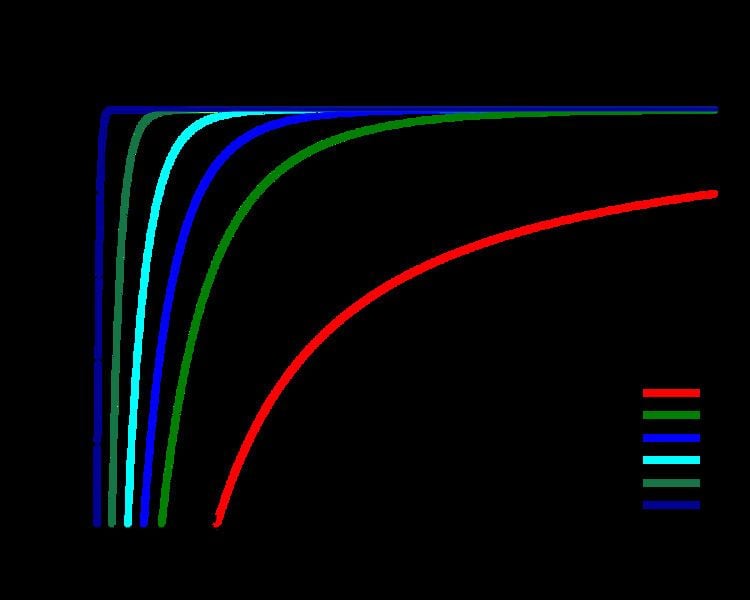
V Coulomb ( r ) = − g 2 1 r . A comparison of the long range potential strength for Yukawa and Coulomb is shown in Figure 2. It can be seen that the Coulomb potential has effect over a greater distance whereas the Yukawa potential approaches zero rather quickly. However, any Yukawa potential or Coulomb potential are non-zero for any large r.
The easiest way to understand that the Yukawa potential is associated with a massive field is by examining its Fourier transform. One has
V ( r ) = − g 2 ( 2 π ) 3 ∫ e i k ⋅ r 4 π k 2 + m 2 d 3 k where the integral is performed over all possible values of the 3-vector momentum k. In this form, the fraction 4 π / ( k 2 + m 2 ) is seen to be the propagator or Green's function of the Klein–Gordon equation.
The Yukawa potential can be derived as the lowest order amplitude of the interaction of a pair of fermions. The Yukawa interaction couples the fermion field ψ ( x ) to the meson field ϕ ( x ) with the coupling term
L i n t ( x ) = g ψ ¯ ( x ) ϕ ( x ) ψ ( x ) . The scattering amplitude for two fermions, one with initial momentum p 1 and the other with momentum p 2 , exchanging a meson with momentum k, is given by the Feynman diagram on the right.
The Feynman rules for each vertex associate a factor of g with the amplitude; since this diagram has two vertices, the total amplitude will have a factor of g 2 . The line in the middle, connecting the two fermion lines, represents the exchange of a meson. The Feynman rule for a particle exchange is to use the propagator; the propagator for a massive meson is − 4 π / ( k 2 + m 2 ) . Thus, we see that the Feynman amplitude for this graph is nothing more than
V ( k ) = − g 2 4 π k 2 + m 2 . From the previous section, this is seen to be the Fourier transform of the Yukawa potential.
The radial Schrödinger equation with Yukawa potential can be solved perturbatively. Using the radial Schrödinger equation in the form
[ d 2 d r 2 + k 2 − l ( l + 1 ) r 2 − V ( r ) ] Ψ ( l , k ; r ) = 0 , and the Yukawa potential in the power-expanded form
V ( r ) = Σ i = − 1 ∞ M i + 1 ( − r ) i , and setting K = i k , one obtains for the angular momentum l the expression
l + n + 1 = − Δ n ( K ) 2 K for | K | → ∞ , where
Δ n ( K ) = M 0 − 1 2 K 2 [ n ( n + 1 ) M 2 + M 0 M 1 ] − ( 2 n + 1 ) M 0 M 2 4 K 3 + 1 8 K 4 [ 3 M 4 ( n − 1 ) n ( n + 1 ) ( n + 2 ) + 2 M 3 M 0 ( 3 n 2 + 3 n − 1 ) + 6 M 2 M 1 n ( n + 1 ) + 2 M 2 M 0 2 + 3 M 1 2 M 0 ] + ( 2 n + 1 ) 8 K 5 [ 3 M 4 M 0 ( n 2 + n − 1 ) + 3 M 3 M 0 2 + M 2 2 n ( n + 1 ) + 4 M 2 M 1 M 0 ] + O ( 1 / K 7 ) . Setting all coefficients M i except M 0 equal to zero, one obtains the well-known expression for the Schrödinger eigenvalue for the Coulomb potential, and the radial quantum number n is a positive integer or zero as a consequence of the boundary conditions which the wave functions of the Coulomb potential have to satisfy. In the case of the Yukawa potential the imposition of boundary conditions is more complicated. Thus in the Yukawa case ν = n is only an approximation and the parameter ν that replaces the integer n is really an asymptotic expansion like that above with first approximation the integer value of the corresponding Coulomb case. The above expansion for the orbital angular momentum or Regge trajectory l ( K ) can be reversed to obtain the energy eigenvalues or equivalently | K | 2 . One obtains:
| K | 2 = − M 1 + M 0 2 4 ( l + n + 1 ) 2 [ 1 − 4 n ( n + 1 ) ( l + n + 1 ) 2 M 2 M 0 + 4 ( 2 n + 1 ) ( l + n + 1 ) 2 M 2 M 0 3 + 4 ( l + n + 1 ) 4 M 0 6 { 3 M 4 M 0 ( n − 1 ) n ( n + 1 ) ( n + 2 ) − 3 M 2 2 n 2 ( n + 1 ) 2 + 2 M 3 M 0 2 ( 3 n 2 + 3 n − 1 ) + 2 M 2 M 0 3 } − 24 ( 2 n + 1 ) ( l + n + 1 ) 5 M 0 6 { M 0 M 4 ( n 2 + n − 1 ) + M 0 3 M 3 − M 2 2 n ( n + 1 ) } − 4 ( l + n + 1 ) 6 M 0 9 { 10 M 6 M 0 2 ( n − 2 ) ( n − 1 ) n ( n + 1 ) ( n + 2 ) ( n + 3 ) + 4 M 3 M 0 5 + 2 M 5 M 0 3 { 5 n ( n + 1 ) ( 3 n 2 + 3 n − 10 ) + 12 } + 2 M 4 M 0 4 ( 6 n 2 + 6 n − 11 ) + 2 M 2 2 M 0 3 ( 9 n 2 + 9 n − 1 ) − 10 M 3 M 2 M 0 2 n ( n + 1 ) ( 3 n 2 + 3 n + 2 ) + 20 M 2 3 n 3 ( n + 1 ) 3 − 30 M 4 M 2 M 0 ( n − 1 ) n 2 ( n + 1 ) 2 ( n + 2 ) } + . . . ] . The above asymptotic expansion of the angular momentum l ( K ) in descending powers of K can also be derived with the WKB method. In that case, however, as in the case of the Coulomb potential the expression l ( l + 1 ) in the centrifugal term of the Schrödinger equation has to be replaced by ( l + 1 / 2 ) 2 , as was argued originally by Langer, the reason being that the singularity is too strong for an unchanged application of the WKB method. That this reasoning is correct follows from the WKB derivation of the correct result in the Coulomb case (with this Langer replacement), and even of the above expansion in the Yukawa case with higher order WKB approximations.