Wiener filter

Description

The goal of the Wiener filter is to compute a statistical estimate of an unknown signal using a related signal as an input and filtering that known signal to produce the estimate as an output. For example, the known signal might consist of an unknown signal of interest that has been corrupted by additive noise. The Wiener filter can be used to filter out the noise from the corrupted signal to provide an estimate of the underlying signal of interest. The Wiener filter is based on a statistical approach, and a more statistical account of the theory is given in the minimum mean square error (MMSE) estimator article.

Typical deterministic filters are designed for a desired frequency response. However, the design of the Wiener filter takes a different approach. One is assumed to have knowledge of the spectral properties of the original signal and the noise, and one seeks the linear time-invariant filter whose output would come as close to the original signal as possible. Wiener filters are characterized by the following:.

1. Assumption: signal and (additive) noise are stationary linear stochastic processes with known spectral characteristics or known autocorrelation and cross-correlation
2. Requirement: the filter must be physically realizable/causal (this requirement can be dropped, resulting in a non-causal solution)
3. Performance criterion: minimum mean-square error (MMSE)

This filter is frequently used in the process of deconvolution; for this application, see Wiener deconvolution.

Wiener filter solutions

The Wiener filter problem has solutions for three possible cases: one where a noncausal filter is acceptable (requiring an infinite amount of both past and future data), the case where a causal filter is desired (using an infinite amount of past data), and the finite impulse response (FIR) case where a finite amount of past data is used. The first case is simple to solve but is not suited for real-time applications. Wiener's main accomplishment was solving the case where the causality requirement is in effect, and in an appendix of Wiener's book Levinson gave the FIR solution.

Noncausal solution

where S are spectral densities. Provided that g ( t ) is optimal, then the minimum mean-square error equation reduces to

and the solution g ( t ) is the inverse two-sided Laplace transform of G ( s ) .

Causal solution

where

This general formula is complicated and deserves a more detailed explanation. To write down the solution G ( s ) in a specific case, one should follow these steps:

1. Start with the spectrum S x ( s ) in rational form and factor it into causal and anti-causal components: S x ( s ) = S x + ( s ) S x − ( s ) where S + contains all the zeros and poles in the left half plane (LHP) and S − contains the zeroes and poles in the right half plane (RHP). This is called the Wiener–Hopf factorization.
2. Divide S x , s ( s ) e α s by S x − ( s ) and write out the result as a partial fraction expansion.
3. Select only those terms in this expansion having poles in the LHP. Call these terms H ( s ) .
4. Divide H ( s ) by S x + ( s ) . The result is the desired filter transfer function G ( s ) .

Finite impulse response Wiener filter for discrete series

The causal finite impulse response (FIR) Wiener filter, instead of using some given data matrix X and output vector Y, finds optimal tap weights by using the statistics of the input and output signals. It populates the input matrix X with estimates of the auto-correlation of the input signal (T) and populates the output vector Y with estimates of the cross-correlation between the output and input signals (V).

In order to derive the coefficients of the Wiener filter, consider the signal w[n] being fed to a Wiener filter of order N and with coefficients { a 0 , ⋯ , a N } . The output of the filter is denoted x[n] which is given by the expression

The residual error is denoted e[n] and is defined as e[n] = x[n] − s[n] (see the corresponding block diagram). The Wiener filter is designed so as to minimize the mean square error (MMSE criteria) which can be stated concisely as follows:

where E [ ⋅ ] denotes the expectation operator. In the general case, the coefficients a i may be complex and may be derived for the case where w[n] and s[n] are complex as well. With a complex signal, the matrix to be solved is a Hermitian Toeplitz matrix, rather than symmetric Toeplitz matrix. For simplicity, the following considers only the case where all these quantities are real. The mean square error (MSE) may be rewritten as:

To find the vector [ a 0 , … , a N ] which minimizes the expression above, calculate its derivative with respect to each a i

Assuming that w[n] and s[n] are each stationary and jointly stationary, the sequences R w [ m ] and R w s [ m ] known respectively as the autocorrelation of w[n] and the cross-correlation between w[n] and s[n] can be defined as follows:

The derivative of the MSE may therefore be rewritten as (notice that R w s [ − i ] = R s w [ i ] )

Letting the derivative be equal to zero results in

which can be rewritten in matrix form

These equations are known as the Wiener–Hopf equations. The matrix T appearing in the equation is a symmetric Toeplitz matrix. Under suitable conditions on R , these matrices are known to be positive definite and therefore non-singular yielding a unique solution to the determination of the Wiener filter coefficient vector, a = T − 1 v . Furthermore, there exists an efficient algorithm to solve such Wiener–Hopf equations known as the Levinson-Durbin algorithm so an explicit inversion of T is not required.

Relationship to the least squares filter

The realization of the causal Wiener filter looks a lot like the solution to the least squares estimate, except in the signal processing domain. The least squares solution, for input matrix X and output vector y is

The FIR Wiener filter is related to the least mean squares filter, but minimizing the error criterion of the latter does not rely on cross-correlations or auto-correlations. Its solution converges to the Wiener filter solution.

Applications

The Wiener filter has a variety of applications in signal processing, image processing, control systems, and digital communications. These applications generally fall into one of four main categories:

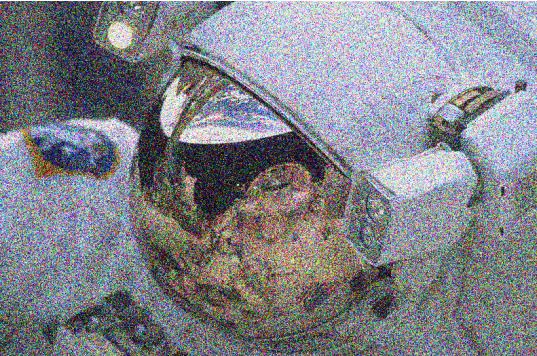
For example, the Wiener filter can be used in image processing to remove noise from a picture. For example, using the Mathematica function: WienerFilter[image,2] on the first image on the right, produces the filtered image below it.

It is commonly used to denoise audio signals, especially speech, as a preprocessor before speech recognition.

History

The filter was proposed by Norbert Wiener during the 1940s and published in 1949. The discrete-time equivalent of Wiener's work was derived independently by Andrey Kolmogorov and published in 1941. Hence the theory is often called the Wiener–Kolmogorov filtering theory (cf. Kriging). The Wiener filter was the first statistically designed filter to be proposed and subsequently gave rise to many others including the Kalman filter.