Walk on spheres method

Informal description

Let Ω be a bounded domain in R d with a sufficiently regular boundary Γ , let h be a function on Γ , and let x be a point inside Ω .

Let us consider the Dirichlet problem:

It can be easily shown that when the solution u exists, for x ∈ Ω :

where W is a d-dimensional Wiener process, the expected value is taken conditionally on {W₀ = x}, and τ is the first-exit time out of Ω.

To compute a solution using this formula, we only have to simulate the first exit point of independent Brownian paths since with the law of large numbers:

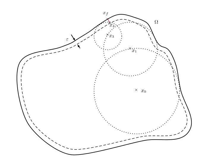
The WoS method provides an efficient way of sampling the first exit point of a Brownian motion from the domain, by remarking that for any (d − 1)-sphere centred on x, the first point of exit of W out of the sphere has a uniform distribution over its surface. Thus, it starts with x⁽⁰⁾ equal to x, and draws the largest sphere S 0 centered on x⁽⁰⁾ and contained inside the domain. The first point of exit x⁽¹⁾ from S 0 is uniformly distributed on its surface. By repeating this step inductively, the WoS provides a sequence (x⁽ⁿ⁾) of positions of the Brownian motion.

According to intuition, the process will converge to the first exit point of the domain. However, this algorithm takes almost surely an infinite number of steps to end. For computational implementation, the process is usually stopped when it gets sufficiently close to the border, and returns the projection of the process on the border. This procedure is sometimes called introducing an ε -shell, or ε -layer.

Formulation of the method

Choose ε > 0 . Using the same notations as above, the Walk-on-spheres algorithm is described as follows:

1. Initialize : x ( 0 ) = x
2. While d ( x ( n ) , Γ ) > ε :
   1. Set r n = d ( x n , Γ ) .
   2. Sample γ n a vector uniformly distributed over the unit sphere, independently from the preceding ones.
   3. Set x ( n + 1 ) := x ( n ) + r n γ n
3. When d ( x ( n ) , Γ ) ≤ ε :
4. x f := p Γ ( x ( n ) ) , the orthogonal projection of x ( n ) on Γ
5. Return x f

The result x f is an estimator of the first exit point from Ω of a Wiener process starting from x , in the sense that they have close probability distributions (see below for comments on the error).

Radius of the spheres

In some cases the distance to the border might be difficult to compute, and it is then preferable to replace the radius of the sphere by a lower bound of this distance. One must then ensure that the radius of the spheres stays large enough so that the process reaches the border.

Bias in the method and GFFP

As it is a Monte-Carlo method, the error of the estimator can be decomposed into the sum of a bias, and a statistical error. The statistical error is reduced by increasing the number of paths sampled, or by using variance reduction methods.

The WoS theoretically provides exact (or unbiased) simulations of the paths of the Brownian motion. However, as it is formulated here, the ε -shell introduced to ensure that the algorithm terminates also adds an error, usually of order O ( ε ) . This error has been studied, and can be avoided in some geometries by using Green's Functions First Passage method: one can change the geometry of the "spheres" when close enough to the border, so that the probability of reaching the border in one step becomes positive. This requires the knowledge of Green's functions for the specific domains. (see also Harmonic measure)

When it is possible to use it, the GFFP method is usually preferred, as it is both faster and more accurate than the classical WoS.

Complexity

It can be shown that the number of steps taken for the WoS process to reach the ε -shell is of order O ( | log ⁡ ( ε ) | ) . Therefore, one can increase the precision to a certain extent without making the number of steps grow notably.

As it is commonly the case for Monte-Carlo methods, this algorithm performs particularly well when the dimension is higher than 3 , and one only needs a small set of values. Indeed, the computational cost increases linearly with the dimension, whereas the cost of grid dependant methods increase exponentially with the dimension.

Variants, extensions

This method has been largely studied, generalized and improved. For example, it is now extensively used for the computation of physical properties of materials (such as capacitance, electrostatic internal energy of molecules, etc.). Some notable extensions include:

Elliptic equations

The WoS method can be modified to solve more general problems. In particular, the method has been generalized to solve Dirichlet problems for equations of the form Δ u = c u + f (which include the Poisson and linearized Poisson−Boltzmann equations) or for any elliptic equation with constant coefficients.

More efficient ways of solving the linearized Poisson–Boltzmann equation have also been developed, relying on Feynman−Kac representations of the solutions.

Time dependency

Again, within a regular enough border, it possible to use the WoS method to solve the following problem :

of which the solution can be represented as:

where the expectation is taken conditionally on X t = x

To use the WoS through this formula, one needs to sample the exit-time from each sphere drawn, which is an independent variable τ 0 with Laplace transform (for a sphere of radius R ):

The total time of exit from the domain τ can be computed as the sum of the exit-times from the spheres. The process also has to be stopped when it has not exited the domain at time T .

Other extensions

The WoS method has been generalized to estimate the solution to elliptic partial differential equations everywhere in a domain, rather than at a single point.

The WoS method has also been generalized in order to compute hitting times for processes other than Brownian motions. For example, hitting times of Bessel processes can be computed via an algorithm called "Walk on moving spheres". This problem has applications in mathematical finance.

Finally, the WoS can be adapted to solve the Poisson and Poisson–Boltzmann equation with flux conditions on the boundary.