Voronoi diagram

Updated on Nov 26, 2024

Edit

Comment

In mathematics, a Voronoi diagram is a partitioning of a plane into regions based on distance to points in a specific subset of the plane. That set of points (called seeds, sites, or generators) is specified beforehand, and for each seed there is a corresponding region consisting of all points closer to that seed than to any other. These regions are called Voronoi cells. The Voronoi diagram of a set of points is dual to its Delaunay triangulation.

It is named after Georgy Voronoi, and is also called a Voronoi tessellation, a Voronoi decomposition, a Voronoi partition, or a Dirichlet tessellation (after Peter Gustav Lejeune Dirichlet). Voronoi diagrams have practical and theoretical applications to a large number of fields, mainly in science and technology but also including visual art. They are also known as Thiessen polygons.

The simplest case

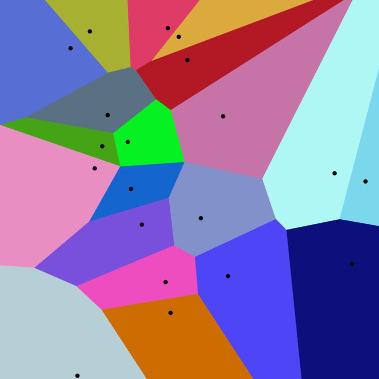
In the simplest case, shown in the first picture, we are given a finite set of points {p₁, …, p_n} in the Euclidean plane. In this case each site p_k is simply a point, and its corresponding Voronoi cell R_k consists of every point in the Euclidean plane whose distance to p_k is less than or equal to its distance to any other p_k. Each such cell is obtained from the intersection of half-spaces, and hence it is a convex polygon. The line segments of the Voronoi diagram are all the points in the plane that are equidistant to the two nearest sites. The Voronoi vertices (nodes) are the points equidistant to three (or more) sites.

Formal definition

Let X be a metric space with distance function d . Let K be a set of indices and let ( P k ) k ∈ K be a tuple (ordered collection) of nonempty subsets (the sites) in the space X . The Voronoi cell, or Voronoi region, R k , associated with the site P k is the set of all points in X whose distance to P k is not greater than their distance to the other sites P j , where j is any index different from k . In other words, if d ( x , A ) = inf { d ( x , a ) ∣ a ∈ A } denotes the distance between the point x and the subset A , then

R k = { x ∈ X ∣ d ( x , P k ) ≤ d ( x , P j ) for all j ≠ k }

The Voronoi diagram is simply the tuple of cells ( R k ) k ∈ K . In principle some of the sites can intersect and even coincide (an application is described below for sites representing shops), but usually they are assumed to be disjoint. In addition, infinitely many sites are allowed in the definition (this setting has applications in geometry of numbers and crystallography), but again, in many cases only finitely many sites are considered.

In the particular case where the space is a finite-dimensional Euclidean space, each site is a point, there are finitely many points and all of them are different, then the Voronoi cells are convex polytopes and they can be represented in a combinatorial way using their vertices, sides, 2-dimensional faces, etc. Sometimes the induced combinatorial structure is referred to as the Voronoi diagram. However, in general the Voronoi cells may not be convex or even connected.

In the usual Euclidean space, we can rewrite the formal definition in usual terms. Each Voronoi polygon R k is associated with a generator point P k . Let X be the set of all points in the Euclidean space. Let P 1 be a point that generates its Voronoi region R 1 , P 2 that generates R 2 , and P 3 that generates R 3 , and so on. Then, as expressed by Tran et al "all locations in the Voronoi polygon are closer to the generator point of that polygon than any other generator point in the Voronoi diagram in Euclidian plane".

Illustration

As a simple illustration, consider a group of shops in a city. Suppose we want to estimate the number of customers of a given shop. With all else being equal (price, products, quality of service, etc.), it is reasonable to assume that customers choose their preferred shop simply by distance considerations: they will go to the shop located nearest to them. In this case the Voronoi cell R k of a given shop P k can be used for giving a rough estimate on the number of potential customers going to this shop (which is modeled by a point in our city).

For most cities, the distance between points can be measured using the familiar Euclidean distance: ℓ 2 = d [ ( a 1 , a 2 ) , ( b 1 , b 2 ) ] = ( a 1 − b 1 ) 2 + ( a 2 − b 2 ) 2 or the Manhattan distance: d [ ( a 1 , a 2 ) , ( b 1 , b 2 ) ] = | a 1 − b 1 | + | a 2 − b 2 | . The corresponding Voronoi diagrams look different for different distance metrics.

Properties

The dual graph for a Voronoi diagram (in the case of a Euclidean space with point sites) corresponds to the Delaunay triangulation for the same set of points.

The closest pair of points corresponds to two adjacent cells in the Voronoi diagram.

Assume the setting is the Euclidean plane and a group of different points are given. Then two points are adjacent on the convex hull if and only if their Voronoi cells share an infinitely long side.

If the space is a normed space and the distance to each site is attained (e.g., when a site is a compact set or a closed ball), then each Voronoi cell can be represented as a union of line segments emanating from the sites. As shown there, this property does not necessarily hold when the distance is not attained.

Under relatively general conditions (the space is a possibly infinite-dimensional uniformly convex space, there can be infinitely many sites of a general form, etc.) Voronoi cells enjoy a certain stability property: a small change in the shapes of the sites, e.g., a change caused by some translation or distortion, yields a small change in the shape of the Voronoi cells. This is the geometric stability of Voronoi diagrams. As shown there, this property does not hold in general, even if the space is two-dimensional (but non-uniformly convex, and, in particular, non-Euclidean) and the sites are points.

History and research

Informal use of Voronoi diagrams can be traced back to Descartes in 1644. Peter Gustav Lejeune Dirichlet used 2-dimensional and 3-dimensional Voronoi diagrams in his study of quadratic forms in 1850. British physician John Snow used a Voronoi diagram in 1854 to illustrate how the majority of people who died in the Broad Street cholera outbreak lived closer to the infected Broad Street pump than to any other water pump.

Voronoi diagrams are named after Russian and Ukrainian mathematician Georgy Fedosievych Voronyi (or Voronoy) who defined and studied the general n-dimensional case in 1908. Voronoi diagrams that are used in geophysics and meteorology to analyse spatially distributed data (such as rainfall measurements) are called Thiessen polygons after American meteorologist Alfred H. Thiessen. In condensed matter physics, such tessellations are also known as Wigner–Seitz unit cells. Voronoi tessellations of the reciprocal lattice of momenta are called Brillouin zones. For general lattices in Lie groups, the cells are simply called fundamental domains. In the case of general metric spaces, the cells are often called metric fundamental polygons. Other equivalent names for this concept (or particular important cases of it): Voronoi polyhedra, Voronoi polygons, domain(s) of influence, Voronoi decomposition, Voronoi tessellation(s), Dirichlet tessellation(s).

Examples

Voronoi tessellations of regular lattices of points in two or three dimensions give rise to many familiar tessellations.

A 2D lattice gives an irregular honeycomb tessellation, with equal hexagons with point symmetry; in the case of a regular triangular lattice it is regular; in the case of a rectangular lattice the hexagons reduce to rectangles in rows and columns; a square lattice gives the regular tessellation of squares; note that the rectangles and the squares can also be generated by other lattices (for example the lattice defined by the vectors (1,0) and (1/2,1/2) gives squares). See here for a dynamic visual example.

A simple cubic lattice gives the cubic honeycomb.

A hexagonal close-packed lattice gives a tessellation of space with trapezo-rhombic dodecahedra.

A face-centred cubic lattice gives a tessellation of space with rhombic dodecahedra.

A body-centred cubic lattice gives a tessellation of space with truncated octahedra.

Parallel planes with regular triangular lattices aligned with each other's centers give the hexagonal prismatic honeycomb.

Certain body centered tetragonal lattices give a tessellation of space with rhombo-hexagonal dodecahedra.

For the set of points (x, y) with x in a discrete set X and y in a discrete set Y, we get rectangular tiles with the points not necessarily at their centers.

Higher-order Voronoi diagrams

Although a normal Voronoi cell is defined as the set of points closest to a single point in S, an nth-order Voronoi cell is defined as the set of points having a particular set of n points in S as its n nearest neighbors. Higher-order Voronoi diagrams also subdivide space.

Higher-order Voronoi diagrams can be generated recursively. To generate the n^th-order Voronoi diagram from set S, start with the (n − 1)^th-order diagram and replace each cell generated by X = {x₁, x₂, ..., x_n−1} with a Voronoi diagram generated on the set S − X.

Farthest-point Voronoi diagram

For a set of n points the (n − 1)^th-order Voronoi diagram is called a farthest-point Voronoi diagram.

For a given set of points S = {p₁, p₂, ..., p_n} the farthest-point Voronoi diagram divides the plane into cells in which the same point of P is the farthest point. A point of P has a cell in the farthest-point Voronoi diagram if and only if it is a vertex of the convex hull of P. Let H = {h₁, h₂, ..., h_k} be the convex hull of P; then the farthest-point Voronoi diagram is a subdivision of the plane into k cells, one for each point in H, with the property that a point q lies in the cell corresponding to a site h_i if and only if d(q, h_i) > d(q, p_j) for each p_j ∈ S with h_i ≠ p_j, where d(p, q) is the Euclidean distance between two points p and q.

The boundaries of the cells in the farthest-point Voronoi diagram have the structure of a topological tree, with infinite rays as its leaves. Every finite tree is isomorphic to the tree formed in this way from a farthest-point Voronoi diagram.

Generalizations and variations

As implied by the definition, Voronoi cells can be defined for metrics other than Euclidean, such as the Mahalanobis distance or Manhattan distance. However, in these cases the boundaries of the Voronoi cells may be more complicated than in the Euclidean case, since the equidistant locus for two points may fail to be subspace of codimension 1, even in the 2-dimensional case.

A weighted Voronoi diagram is the one in which the function of a pair of points to define a Voronoi cell is a distance function modified by multiplicative or additive weights assigned to generator points. In contrast to the case of Voronoi cells defined using a distance which is a metric, in this case some of the Voronoi cells may be empty. A power diagram is a type of Voronoi diagram defined from a set of circles using the power distance; it can also be thought of as a weighted Voronoi diagram in which a weight defined from the radius of each circle is added to the squared distance from the circle's center.

The Voronoi diagram of n points in d-dimensional space requires O ( n ⌈ 1 2 d ⌉ ) storage space. Therefore, Voronoi diagrams are often not feasible for d > 2. An alternative is to use approximate Voronoi diagrams, where the Voronoi cells have a fuzzy boundary, which can be approximated. Another alternative is when any site is a fuzzy circle and as a result the cells become fuzzy too.

Voronoi diagrams are also related to other geometric structures such as the medial axis (which has found applications in image segmentation, optical character recognition, and other computational applications), straight skeleton, and zone diagrams. Besides points, such diagrams use lines and polygons as seeds. By augmenting the diagram with line segments that connect to nearest points on the seeds, a planar subdivision of the environment is obtained. This structure can be used as a navigation mesh for path-finding through large spaces. The navigation mesh has been generalized to support 3D multi-layered environments, such as an airport or a multi-storey building.

Natural sciences

In biology, Voronoi diagrams are used to model a number of different biological structures, including cells and bone microarchitecture. Indeed, Voronoi tessellations work as a geometrical tool to understand the physical constraints that drive the organization of biological tissues.

In hydrology, Voronoi diagrams are used to calculate the rainfall of an area, based on a series of point measurements. In this usage, they are generally referred to as Thiessen polygons.

In ecology, Voronoi diagrams are used to study the growth patterns of forests and forest canopies, and may also be helpful in developing predictive models for forest fires.

In computational chemistry, Voronoi cells defined by the positions of the nuclei in a molecule are used to compute atomic charges. This is done using the Voronoi deformation density method.

In astrophysics, Voronoi diagrams are used to generate adaptative smoothing zones on images, adding signal fluxes on each one. The main objective for these procedures is to maintain a relatively constant signal-to-noise ratio on all the image.

In computational fluid dynamics, the Voronoi tessellation of a set of points can be used to define the computational domains used in finite volume methods, e.g. as in the moving-mesh cosmology code AREPO.

Health

In medical diagnosis, Voronoi diagrams-based models for muscle tissue can be used to detect neuromuscular diseases.

In epidemiology, Voronoi diagrams can be used to correlate sources of infections in epidemics. One of the early applications of Voronoi diagrams was implemented by John Snow to study the 1854 Broad Street cholera outbreak in Soho, England. He showed the correlation between residential areas on the map of Central London whose residents had been using a specific water pump, and the areas with most deaths due to the outbreak.

Engineering

In polymer physics, Voronoi diagrams can be used to represent free volumes of polymers.

In materials science, polycrystalline microstructures in metallic alloys are commonly represented using Voronoi tessellations. In solid state physics, the Wigner-Seitz cell is the Voronoi tessellation of a solid, and the Brillouin zone is the Voronoi tessellation of reciprocal (wave number) space of crystals which have the symmetry of a space group.

In aviation, Voronoi diagrams are superimposed on oceanic plotting charts to identify the nearest airfield for in-flight diversion (see ETOPS), as an aircraft progresses through its flight plan.

In architecture, Voronoi patterns were the basis for the winning entry for redevelopment of The Arts Centre Gold Coast.

In mining, Voronoi polygons are used to estimate the reserves of valuable materials, minerals, or other resources. Exploratory drillholes are used as the set of points in the Voronoi polygons.

Geometry

A point location data structure can be built on top of the Voronoi diagram in order to answer nearest neighbor queries, where one wants to find the object that is closest to a given query point. Nearest neighbor queries have numerous applications. For example, one might want to find the nearest hospital, or the most similar object in a database. A large application is vector quantization, commonly used in data compression.

In geometry, Voronoi diagrams can be used to find the largest empty circle amid a set of points, and in an enclosing polygon; e.g. to build a new supermarket as far as possible from all the existing ones, lying in a certain city.

Voronoi diagrams together with farthest-point Voronoi diagrams are used for efficient algorithms to compute the roundness of a set of points. The Voronoi approach is also put to good use in the evaluation of circularity/roundness while assessing the dataset from a coordinate-measuring machine.

Informatics

In networking, Voronoi diagrams can be used in derivations of the capacity of a wireless network.

In computer graphics, Voronoi diagrams are used to calculate 3D shattering / fracturing geometry patterns. It is also used to procedurally generate organic or lava-looking textures.

In autonomous robot navigation, Voronoi diagrams are used to find clear routes. If the points are obstacles, then the edges of the graph will be the routes furthest from obstacles (and theoretically any collisions).

In machine learning, Voronoi diagrams are used to do 1-NN classifications.

In user interface development, Voronoi patterns can be used to compute the best hover state for a given point.

Algorithms

Direct algorithms:

Fortune's algorithm, an O(n log(n)) algorithm for generating a Voronoi diagram from a set of points in a plane.

Lloyd's algorithm and its generalization via the Linde–Buzo–Gray algorithm (aka k-means clustering), produces a Voronoi tessellation in a space of arbitrary dimensions.

Starting with a Delaunay triangulation (obtain the dual):

Bowyer–Watson algorithm, an O(n log(n)) to O(n²) algorithm for generating a Delaunay triangulation in any number of dimensions, from which the Voronoi diagram can be obtained.

References

Voronoi diagram Wikipedia

(Text) CC BY-SA

Contents