Visibility polygon

Definitions

Formally, we can define the planar visibility polygon problem as such. Let S be a set of obstacles (either segments, or polygons) in R 2 . Let p be a point in R 2 that is not within an obstacle. Then, the point visibility polygon V is the set of points in R 2 , such that for every point q in V , the segment p q does not intersect any obstacle in S .

Likewise, the segment visibility polygon or edge visibility polygon is the portion visible to any point along a line segment.

Applications

Visibility polygons are useful in robotics. For example, in robot localization, a robot using sensors such as a lidar will detect obstacles that it can see, which is similar to a visibility polygon.

They are also useful in video games, with numerous online tutorials explaining simple algorithms for implementing it.

Algorithms for point visibility polygons

Numerous algorithms have been proposed for computing the point visibility polygon. For different variants of the problem (e.g. different types of obstacles), algorithms vary in time complexity.

Naive algorithms

Naive algorithms are easy to understand and implement, but they are not optimal, since they can be much slower than other algorithms.

Uniform ray casting "physical" algorithm

In real life, a glowing point illuminates the region visible to it because it emits light in every direction. This can be simulated by shooting rays in many directions. Suppose that the point is p and the set of obstacles is S . Then, the pseudocode may be expressed in the following way:

Algorithm naive_bad_algorithm( p , S ) V := ∅ for θ = 0 , ⋯ , 2 π : // shoot a ray with angle θ r := ∞ for each obstacle in S : r := min( r , distance from p to the obstacle in this direction) add vertex ( θ , r ) to V return V

Now, if it were possible to try all the infinitely many angles, the result would be correct. Unfortunately, it is impossible to really try every single direction due to the limitations of computers. An approximation can be created by casting many, say, 50 rays spaced uniformly apart. However, this is not an exact solution, since small obstacles might be missed by two adjacent rays entirely. Furthermore, it is very slow, since one may have to shoot many rays to gain a roughly similar solution, and the output visibility polygon may have many more vertices in it than necessary.

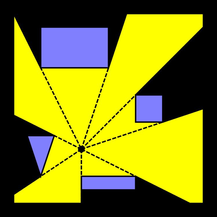
Ray casting to every vertex

The previously described algorithm can be significantly improved in both speed and correctness by making the observation that it suffices to only shoot rays to every obstacle's vertices. This is because any bends or corners along the boundary of a visibility polygon must be due to some corner (i.e. a vertex) in an obstacle.

Algorithm naive_better_algorithm( p , S ) V := ∅ for each obstacle b in S : for each vertex v of b : // shoot a ray from p to v r := distance from p to v θ := angle of v with respect to p for each obstacle b ′ in S : r := min( r , distance from p to b ′ ) add vertex ( θ , r ) to V return V

The time complexity of this algorithm is O ( n 2 ) . This is because the algorithm shoots a ray to every one of the n vertices, and to check where the ray ends, it has to check for intersection with every one of the O ( n ) obstacles. This is sufficient for many simple applications such as video games, and as such many online tutorials teach this method. However, as we shall see later, there are faster O ( n log ⁡ n ) algorithms (or even faster ones if the obstacle is a simple polygon or if there are a fixed number of polygonal holes).

Optimal algorithms for a point in a simple polygon

Given a simple polygon P and a point p , a linear time algorithm is optimal for computing the region in P that is visible from p . Such an algorithm was first proposed in 1981. However, it is quite complicated. In 1983, a conceptually simpler algorithm was proposed, which had a minor error that was corrected in 1987.

The latter algorithm will be briefly explained here. It simply walks around the boundary of the polygon P , processing the vertices in the order in which they appear, while maintaining a stack of vertices S = s 0 , s 1 , ⋯ , s t where s t is the top of the stack. The stack constitutes the vertices encountered so far which are visible to p . If, later during the execution of the algorithm, some new vertices are encountered that obscure part of S , then the obscured vertices in S will be popped from the stack. By the time the algorithm terminates, S will consist of all the visible vertices, i.e. the desired visibility polygon. An efficient implementation was published in 2014.

Optimal algorithms for a point in a polygon with holes

For a point in a polygon with h holes and n vertices in total, it can be shown that in the worst case, a Θ ( n + h log ⁡ h ) algorithm is optimal. Such an algorithm was proposed in 1995 together with its proof of optimality. However, it relies on the linear time polygon triangulation algorithm by Chazelle, which is extremely complex.

Segments that do not intersect except at their endpoints

For a point among a set of n segments that do not intersect except at their endpoints, it can be shown that in the worst case, a Θ ( n log ⁡ n ) algorithm is optimal. This is because a visibility polygon algorithm must output the vertices of the visibility polygon in sorted order, hence the problem of sorting can be reduced to computing a visibility polygon.

Notice that any algorithm that computes a visibility polygon for a point among segments can be used to compute a visibility polygon for all other kinds of polygonal obstacles, since any polygon can be decomposed into segments.

Divide and conquer

A divide and conquer algorithm to compute the visibility polygon was proposed in 1987.

Angular sweep

An angular sweep, i.e. rotational plane sweep algorithm to compute the visibility polygon was proposed in 1985 and 1986. The idea is to first sort all the segment endpoints by polar angle, and then iterate over them in that order. During the iteration, the event line is maintained as a heap. An efficient implementation was published in 2014.

Generally intersecting segments

For a point among generally intersecting segments, the visibility polygon problem is reducible, in linear time, to the lower envelope problem. By the Davenport–Schinzel argument, the lower envelope in the worst case has Θ ( n α ( n ) ) number of vertices, where α ( n ) is the inverse Ackermann function. A worst case optimal divide-and-conquer algorithm running in Θ ( n log ⁡ n ) time was created by John Hershberger in 1989.