Vibration of plates - Alchetron, The Free Social Encyclopedia

The vibration of plates is a special case of the more general problem of mechanical vibrations. The equations governing the motion of plates are simpler than those for general three-dimensional objects because one of the dimensions of a plate is much smaller than the other two. This suggests that a two-dimensional plate theory will give an excellent approximation to the actual three-dimensional motion of a plate-like object, and indeed that is found to be true.

There are several theories that have been developed to describe the motion of plates. The most commonly used are the Kirchhoff-Love theory and the Mindlin-Reissner theory. Solutions to the governing equations predicted by these theories can give us insight into the behavior of plate-like objects both under free and forced conditions. This includes the propagation of waves and the study of standing waves and vibration modes in plates.

Kirchhoff-Love plates

The governing equations for the dynamics of a Kirchhoff-Love plate are

N α β , β = J 1 u ¨ α M α β , α β − q ( x , t ) = J 1 w ¨ − J 3 w ¨ , α α

where u α are the in-plane displacements of the mid-surface of the plate, w is the transverse (out-of-plane) displacement of the mid-surface of the plate, q is an applied transverse load, and the resultant forces and moments are defined as

N α β := ∫ − h h σ α β d x 3 and M α β := ∫ − h h x 3 σ α β d x 3 .

Note that the thickness of the plate is 2 h and that the resultants are defined as weighted averages of the in-plane stresses σ α β . The derivatives in the governing equations are defined as

u ˙ i := ∂ u i ∂ t ; u ¨ i := ∂ 2 u i ∂ t 2 ; u i , α := ∂ u i ∂ x α ; u i , α β := ∂ 2 u i ∂ x α ∂ x β

where the Latin indices go from 1 to 3 while the Greek indices go from 1 to 2. Summation over repeated indices is implied. The x 3 coordinates is out-of-plane while the coordinates x 1 and x 2 are in plane. For a uniformly thick plate of thickness 2 h and homogeneous mass density ρ

J 1 := ∫ − h h ρ d x 3 = 2 ρ h and J 3 := ∫ − h h x 3 2 ρ d x 3 = 2 3 ρ h 3 .

Isotropic Kirchhoff–Love plates

For an isotropic and homogeneous plate, the stress-strain relations are

[ σ 11 σ 22 σ 12 ] = E 1 − ν 2 [ 1 ν 0 ν 1 0 0 0 1 − ν ] [ ε 11 ε 22 ε 12 ] .

where ε α β are the in-plane strains. The strain-displacement relations for Kirchhoff-Love plates are

ε α β = 1 2 ( u α , β + u β , α ) − x 3 w , α β .

Therefore, the resultant moments corresponding to these stresses are

[ M 11 M 22 M 12 ] = − 2 h 3 E 3 ( 1 − ν 2 ) [ 1 ν 0 ν 1 0 0 0 1 − ν ] [ w , 11 w , 22 w , 12 ]

If we ignore the in-plane displacements u α β , the governing equations reduce to

D ∇ 2 ∇ 2 w = − q ( x , t ) − 2 ρ h w ¨ where D is the bending stiffness of the plate. For a uniform plate of thickness 2 h , D := 2 h 3 E 3 ( 1 − ν 2 ) .

The above equation can also be written in an alternative notation:

μ Δ Δ w + q ^ + ρ w t t = 0 .

In solid mechanics, a plate is often modeled as a two-dimensional elastic body whose potential energy depends on how it is bent from a planar configuration, rather than how it is stretched (which is the instead the case for a membrane such as a drumhead). In such situations, a vibrating plate can be modeled in a manner analogous to a vibrating drum. However, the resulting partial differential equation for the vertical displacement w of a plate from its equilibrium position is fourth order, involving the square of the Laplacian of w, rather than second order, and its qualitative behavior is fundamentally different from that of the circular membrane drum.

Free vibrations of isotropic plates

For free vibrations, the external force q is zero, and the governing equation of an isotropic plate reduces to

D ∇ 2 ∇ 2 w = − 2 ρ h w ¨

or

μ Δ Δ w + ρ w t t = 0 .

This relation can be derived in an alternative manner by considering the curvature of the plate. The potential energy density of a plate depends how the plate is deformed, and so on the mean curvature and Gaussian curvature of the plate. For small deformations, the mean curvature is expressed in terms of w, the vertical displacement of the plate from kinetic equilibrium, as Δw, the Laplacian of w, and the Gaussian curvature is the Monge–Ampère operator w_xxw_yy−w2
xy. The total potential energy of a plate Ω therefore has the form

U = ∫ Ω [ ( Δ w ) 2 + ( 1 − μ ) ( w x x w y y − w x y 2 ) ] d x d y

apart from an overall inessential normalization constant. Here μ is a constant depending on the properties of the material.

The kinetic energy is given by an integral of the form

T = ρ 2 ∫ Ω w t 2 d x d y .

Hamilton's principle asserts that w is a stationary point with respect to variations of the total energy T+U. The resulting partial differential equation is

ρ w t t + μ Δ Δ w = 0.

Circular plates

For freely vibrating circular plates, w = w ( r , t ) , and the Laplacian in cylindrical coordinates has the form

∇ 2 w ≡ 1 r ∂ ∂ r ( r ∂ w ∂ r ) .

Therefore, the governing equation for free vibrations of a circular plate of thickness 2 h is

1 r ∂ ∂ r [ r ∂ ∂ r { 1 r ∂ ∂ r ( r ∂ w ∂ r ) } ] = − 2 ρ h D ∂ 2 w ∂ t 2 .

Expanded out,

∂ 4 w ∂ r 4 + 2 r ∂ 3 w ∂ r 3 − 1 r 2 ∂ 2 w ∂ r 2 + 1 r 3 ∂ w ∂ r = − 2 ρ h D ∂ 2 w ∂ t 2 .

To solve this equation we use the idea of separation of variables and assume a solution of the form

w ( r , t ) = W ( r ) F ( t ) .

Plugging this assumed solution into the governing equation gives us

1 β W [ d 4 W d r 4 + 2 r d 3 W d r 3 − 1 r 2 d 2 W d r 2 + 1 r 3 d W d r ] = − 1 F d 2 F d t 2 = ω 2

where ω 2 is a constant and β := 2 ρ h / D . The solution of the right hand equation is

F ( t ) = Re [ A e i ω t + B e − i ω t ] .

The left hand side equation can be written as

d 4 W d r 4 + 2 r d 3 W d r 3 − 1 r 2 d 2 W d r 2 + 1 r 3 d W d r = λ 4 W

where λ 4 := β ω 2 . The general solution of this eigenvalue problem that is appropriate for plates has the form

W ( r ) = C 1 J 0 ( λ r ) + C 2 I 0 ( λ r )

where J 0 is the order 0 Bessel function of the first kind and I 0 is the order 0 modified Bessel function of the first kind. The constants C 1 and C 2 are determined from the boundary conditions. For a plate of radius a with a clamped circumference, the boundary conditions are

W ( r ) = 0 and d W d r = 0 at r = a .

From these boundary conditions we find that

J 0 ( λ a ) I 1 ( λ a ) + I 0 ( λ a ) J 1 ( λ a ) = 0 .

We can solve this equation for λ n (and there are an infinite number of roots) and from that find the modal frequencies ω n = λ n 2 / β . We can also express the displacement in the form

w ( r , t ) = ∑ n = 1 ∞ C n [ J 0 ( λ n r ) − J 0 ( λ n a ) I 0 ( λ n a ) I 0 ( λ n r ) ] [ A n e i ω n t + B n e − i ω n t ] .

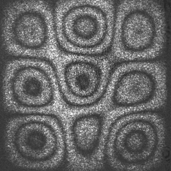
For a given frequency ω n the first term inside the sum in the above equation gives the mode shape. We can find the value of C 1 using the appropriate boundary condition at r = 0 and the coefficients A n and B n from the initial conditions by taking advantage of the orthogonality of Fourier components.

Rectangular plates

Consider a rectangular plate which has dimensions a × b in the ( x 1 , x 2 ) -plane and thickness 2 h in the x 3 -direction. We seek to find the free vibration modes of the plate.

Assume a displacement field of the form

w ( x 1 , x 2 , t ) = W ( x 1 , x 2 ) F ( t ) .

Then,

∇ 2 ∇ 2 w = w , 1111 + 2 w , 1212 + w , 2222 = [ ∂ 4 W ∂ x 1 4 + 2 ∂ 4 W ∂ x 1 2 ∂ x 2 2 + ∂ 4 W ∂ x 2 4 ] F ( t )

and

w ¨ = W ( x 1 , x 2 ) d 2 F d t 2 .

Plugging these into the governing equation gives

D 2 ρ h W [ ∂ 4 W ∂ x 1 4 + 2 ∂ 4 W ∂ x 1 2 ∂ x 2 2 + ∂ 4 W ∂ x 2 4 ] = − 1 F d 2 F d t 2 = ω 2

where ω 2 is a constant because the left hand side is independent of t while the right hand side is independent of x 1 , x 2 . From the right hand side, we then have

F ( t ) = A e i ω t + B e − i ω t .

From the left hand side,

∂ 4 W ∂ x 1 4 + 2 ∂ 4 W ∂ x 1 2 ∂ x 2 2 + ∂ 4 W ∂ x 2 4 = 2 ρ h ω 2 D W =: λ 4 W

where

λ 2 = ω 2 ρ h D .

Since the above equation is a biharmonic eigenvalue problem, we look for Fourier expansion solutions of the form

W m n ( x 1 , x 2 ) = sin ⁡ m π x 1 a sin ⁡ n π x 2 b .

We can check and see that this solution satisfies the boundary conditions for a freely vibrating rectangular plate with simply supported edges:

w ( x 1 , x 2 , t ) = 0 at x 1 = 0 , a and x 2 = 0 , b M 11 = D ( ∂ 2 w ∂ x 1 2 + ν ∂ 2 w ∂ x 2 2 ) = 0 at x 1 = 0 , a M 22 = D ( ∂ 2 w ∂ x 2 2 + ν ∂ 2 w ∂ x 1 2 ) = 0 at x 2 = 0 , b .

Plugging the solution into the biharmonic equation gives us

λ 2 = π 2 ( m 2 a 2 + n 2 b 2 ) .

Comparison with the previous expression for λ 2 indicates that we can have an infinite number of solutions with

ω m n = ( m 2 a 2 + n 2 b 2 ) D π 4 2 ρ h .

Therefore the general solution for the plate equation is

w ( x 1 , x 2 , t ) = ∑ m = 1 ∞ ∑ n = 1 ∞ sin ⁡ m π x 1 a sin ⁡ n π x 2 b ( A m n e i ω m n t + B m n e − i ω m n t ) .

To find the values of A m n and B m n we use initial conditions and the orthogonality of Fourier components. For example, if

w ( x 1 , x 2 , 0 ) = φ ( x 1 , x 2 ) on x 1 ∈ [ 0 , a ] and ∂ w ∂ t ( x 1 , x 2 , 0 ) = ψ ( x 1 , x 2 ) on x 2 ∈ [ 0 , b ]

we get,

A m n = 4 a b ∫ 0 a ∫ 0 b φ ( x 1 , x 2 ) sin ⁡ m π x 1 a sin ⁡ n π x 2 b d x 1 d x 2 B m n = 4 a b ω m n ∫ 0 a ∫ 0 b ψ ( x 1 , x 2 ) sin ⁡ m π x 1 a sin ⁡ n π x 2 b d x 1 d x 2 .

References

Vibration of plates Wikipedia

(Text) CC BY-SA

Similar TopicsThe Sorrows of Satan (film)

Disappearance of Revelle Balmain

Jessica Chobot