Two state quantum system - Alchetron, the free social encyclopedia

In quantum mechanics, a two-state system (also known as a two-level system) is a system that can exist in any quantum superposition of two independent (physically distinguishable) quantum states. The Hilbert space describing such a system is two-dimensional. Therefore, a complete basis spanning the space will consist of two independent states.

Two-state systems are the simplest quantum systems that can exist, since the dynamics of a one-state system is trivial (i.e. there is no other state the system can exist in). The mathematical framework required for the analysis of two-state systems is that of linear differential equations and linear algebra of two-dimensional spaces. As a result, the dynamics of a two-state system can be solved analytically without any approximation.

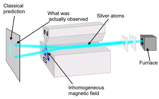
A very well known example of a two-state system is the spin of a spin-1/2 particle such as an electron, whose spin can have values +ħ/2 or −ħ/2, where ħ is the reduced Planck constant. Another example, frequently studied in atomic physics, is the transition of an atom to or from an excited state; here the two-state formalism is used to quantitatively explain stimulated and spontaneous emission of photons from excited atoms.

Representation of the Two-state quantum system

The state of a two-state quantum system can be described by a two-dimensional complex Hilbert space, this means every state vector | ψ ⟩ is represented by two complex coordinates.

| ψ ⟩ = ( c 1 c 2 ) = c 1 ( 1 0 ) + c 2 ( 0 1 ) ; where, c 1 and c 2 are the coordinates.

If the vectors are normalized, c 1 and c 2 are related by | c 1 | 2 + | c 2 | 2 = 1 . the basis vectors will be represented as | 0 ⟩ = ( 1 0 ) and | 1 ⟩ = ( 0 1 )

All observable physical quantities associated with this systems are 2 × 2 Hermitian matrices, this means the Hamiltonian of the system is also a similar matrix.

The Two-state Hamiltonian

The most general form of the Hamiltonian of a two-state system is given

H = ( a 1 c − i d c + i d a 2 )

here, a 1 , a 2 , c and d are real numbers. This matrix can be decomposed as,

H = a ⋅ σ 0 + c ⋅ σ 1 + d ⋅ σ 2 + b ⋅ σ 3 ;

Here, a = ( a 1 + a 2 ) 2 and b = ( a 1 − a 2 ) 2 are real numbers. The matrix σ 0 is the 2 × 2 identity matrix and the matrices σ k ( k = 1 , 2 , 3 ) are the Pauli matrices. This decomposition simplifies the analysis of the system especially in the time-independent case where the values of a , b , c and d are constants.

The Hamiltonian can be written (in a slightly different vector form) as:

H = a ⋅ σ 0 + r ⋅ σ ;

The vector r is given by ( c , d , b ) and σ is given by ( σ 1 , σ 2 , σ 3 ) . This representation simplifies the analysis of the time evolution of the system and is easier to use with other specialized representations such as the Bloch sphere.

Eigenvalues of the Hamiltonian, Basis vectors and Time evolution

Let H be the time-independent Hamiltonian of a two-state system, the Eigenvalues are given by E ± = a ± | r | and the eigenvectors corresponding to them are given as | E + ⟩ and | E − ⟩ corresponding to their respective energies. When one changes the basis to the eigenvectors the Hamiltonian is diagonal and is of the form,

H = ( E + 0 0 E − ) ;

the unitary time evolution operator U is given by:

U ( t ) = e − i H t ℏ = e − i a t ℏ ( cos ⁡ ( | r | ) σ 0 + i sin ⁡ ( | r | ) r ^ ⋅ σ ) ;

where, r ^ = r | r | . . This is the case when H is in the vector form (i.e. in the | 0 ⟩ , | 1 ⟩ basis); in the eigenvector basis U is diagonal and is given by:

U ( t ) = ( e − i E + t ℏ 0 0 e − i E − t ℏ )

It is to be noted that the e − i a t ℏ factor only contributes to the overall phase of the operator and can therefore be ignored to yield a new time evolution operator that is physically indistinguishable from the original operator. Moreover, any perturbation to the system (which will be of the same form as the Hamiltonian) can be added to the system in the eigenbasis of the unperturbed Hamiltonian and analysed in the same way as above, this means that for any perturbation the new eigenvectors of the perturbed system can be solved exactly (as mentioned in the introduction).

Dynamics of the Two-state System: The Rabi formula

If H is the time-independent Hamiltonian, let | + ⟩ and | − ⟩ denote the two energy eigenstates of the system, with respective eigenvalues E + and E − . Any state | ψ ( t ) ⟩ of the two-level system can be written as a superposition of the energy eigenstates; in particular, at time t = 0 we can write,

| ψ ( 0 ) ⟩ = c + | + ⟩ + c − | − ⟩ ,

the above vector is assumed to be normalized. The time evolution of the state | ψ ( 0 ) ⟩ is given by the relation

| ψ ( t ) ⟩ = U ( t ) | ψ ( 0 ) ⟩ = c + e − i E + t ℏ | + ⟩ + c − e − i E − t ℏ | − ⟩ ,

further eliminating an overall phase factor of e − i E + t ℏ the time evolved state can be represented as,

| ψ ( t ) ⟩ = c + | + ⟩ + c − e − i ( E − − E + ) t ℏ | − ⟩ ,

It is easy to infer that if the system was initially in one of the eigestates ( | + ⟩ or | − ⟩ ) it will continue to remain in the same state, however in a general state as shown above the time evolution is non-trivial. Upon calculating the probability of the state returning to the initial state at a given time t is given by

| ⟨ ψ ( 0 ) | ψ ( t ) ⟩ | 2 = | | c + | 2 + | c − | 2 e − i ( E − − E + ) t ℏ | 2 = 1 − 4 | c + c − | 2 sin 2 ( ω t 2 )

Where ω is a characteristic angular frequency given by

ω = E + − E − ℏ ,

where it has been assumed that E + ≥ E − .

It can be seen that the probability of finding the system in its initial quantum state oscillates between 1 − 4 | c + c − | 2 and 1 this formula is called the Rabi oscillation formula. In the case E + = E − , that is when the Hamiltonian is degenerate there is no oscillation.

Precession in a field

Consider the case of a spin-1/2 particle in a magnetic field B = B n ^ . The interaction Hamiltonian for this system is

H = − μ ⋅ B = − μ σ ⋅ B

where μ is the magnitude of the particle's magnetic moment and σ is the vector of Pauli matrices. Solving the time dependent Schrödinger equation H ψ = i ℏ ∂ t ψ yields

ψ ( t ) = e i ω t σ ⋅ n ^ ψ ( 0 ) ,

where ω = μ B / ℏ and e i ω t σ ⋅ n ^ = cos ⁡ ( ω t ) I + i n ^ ⋅ σ sin ⁡ ( ω t ) . Physically, this corresponds to the Bloch vector precessing around n ^ with angular frequency 2 ω . Without loss of generality, assume the field is uniform points in z ^ , so that the time evolution operator is given as

e i ω t σ ⋅ n ^ = ( e i ω t 0 0 e − i ω t ) .

It can be seen that such a time evolution operator acting on a general spin state of a spin-1/2 particle will lead to the precession about the axis defined by the applied magnetic field (this is the quantum mechanical equivalent of Larmor precession)

The above method can however be applied to the analysis of any generic two-state system that is interacting with some field (equivalent to the magnetic field in the previous case) the interaction is given by an appropriate coupling term that is analogous to the magnetic moment. The precession of the state vector (which need not be a physical spinning as in the previous case) can be viewed as the precession of the state vector on the Bloch sphere

The representation on the Bloch sphere for a state vector ψ ( 0 ) will simply be the vector of expectation values R = ( ⟨ σ x ⟩ , ⟨ σ y ⟩ , ⟨ σ z ⟩ ) . As an example, consider a state vector ψ ( 0 ) that is a normalized superposition of | ↑ ⟩ and | ↓ ⟩ , that is, a vector that can be represented in the σ z basis as

ψ ( 0 ) = 1 2 ( 1 1 )

The components of ψ ( t ) on the Bloch sphere will simply be R = ( cos ⁡ 2 ω t , − sin ⁡ 2 ω t , 0 ) . This is a unit vector that begins pointing along x ^ and precesses around z ^ in a left-handed manner. In general, by a rotation around z ^ , any state vector ψ ( 0 ) can be represented as a | ↑ ⟩ + b | ↓ ⟩ with real coefficients a and b . Such a state vector corresponds to a Bloch vector in the xz-plane making an angle tan ⁡ ( θ / 2 ) = b / a with the z-axis. This vector will proceed to precess around z ^ . In theory, by allowing the system to interact with the field of a particular direction and strength for precise durations, it is possible to obtain any orientation of the Bloch vector, which is equivalent to obtaining any complex superposition. This is the basis for numerous technologies including quantum computing and MRI.

Evolution in a Time-dependent Field: Nuclear magnetic resonance

Nuclear magnetic resonance (NMR) is an important example in the dynamics of two-state systems because it is involves the exact solution to a time dependent Hamiltonian. The NMR phenomenon is achieved by placing a nucleus in a strong, static field B₀ (the "holding field") and then applying a weak, transverse field B₁ that oscillates at some radiofrequency ω_r. Explicitly, consider a spin-1/2 particle in a holding field B 0 z ^ and a transverse rf field B₁ rotating in the xy-plane in a right-handed fashion around B₀:

As in the free precession case, the Hamiltonian is H = − μ σ ⋅ B , and the evolution of a state vector ψ ( t ) is found by solving the time-dependent Schrödinger equation H ψ = i ℏ ∂ ψ / ∂ t . After some manipulation (given in the collapsed section below), it can be shown that the Schrödinger equation becomes

∂ ψ ∂ t = i ( ω 1 σ x + ( w 0 + ω r 2 ) σ z ) ψ ,

where ω 0 = μ B 0 / ℏ and ω 1 = μ B 1 / ℏ .

As per the previous section, the solution to this equation has the Bloch vector precessing around ( ω 1 , 0 , ω 0 + ω r / 2 ) with a frequency that is twice the magnitude of the vector. If ω 0 is sufficiently strong, some proportion of the spins will be pointing directly down prior to the introduction of the rotating field. If the angular frequency of the rotating magnetic field is chosen such that ω r = − 2 ω 0 , in the rotating frame the state vector will precess around x ^ with frequency 2 ω 1 , and will thus flip from down to up releasing energy in the form of detectable photons. This is the fundamental basis for NMR, and in practice is accomplished by scanning ω r until the resonant frequency is found at which point the sample will emit light. Similar calculations are done in atomic physics, and in the case that the field is not rotating, but oscillating with a complex amplitude, use is made of the rotating wave approximation in deriving such results.

Relation to Bloch equations

The optical Bloch equations for a collection of spin-1/2 particles can be derived from the time dependent Schrödinger equation for a two level system. Starting with the previously stated Hamiltonian i ℏ ∂ t ψ = − μ σ → ⋅ B → ψ , it can be written in summation notation after some rearrangement as

Multiplying by a Pauli matrix σ i and the conjugate transpose of the wavefunction, and subsequently expanding the product of two Pauli matrices yields

Adding this equation to its own conjugate transpose yields a left hand side of the form

And a right hand side of the form

As previously mentioned, the expectation value of each Pauli matrix is a component of the Bloch vector, ⟨ σ i ⟩ = ψ † σ i ψ = R i . Equating the left and right hand sides, and noting that 2 μ ℏ is the gyromagnetic ratio γ , yields another form for the equations of motion of the Bloch vector

where the fact that ε i j k = ε k i j has been used. In vector form these three equations can be expressed in terms of a cross product

Classically, this equation describes the dynamics of a spin in a magnetic field. An ideal magnet consists of a collection of identical spins behaving independently, and thus the total magnetization M → is proportional to the Bloch vector R → . All that is left to obtain the final form of the optical Bloch equations is the inclusion of the phenomenological relaxation terms.

As a final aside, the above equation can be derived by considering the time evolution of the angular momentum operator in the Heisenberg picture.

Which, when coupled with the fact that R i → = ⟨ σ i ⟩ , is the same equation as before.

The Validity of the Two-state formalism

Two-state systems are the simplest non-trivial quantum systems that occur in nature however it should be noted that the above mentioned methods of analysis are not just valid for simple two-state systems. Any general multi-state quantum system can be effectively treated as two-state system as long as a particular property of is being considered (which behaves as a two-state system) an example of this that of a spin-1/2 particle, which may have additional translational or even rotational degrees of freedom, however in the preceding analysis, the additional degrees freedom are ignored.

Another case where the effective two-state formalism is valid is when the system under consideration has two levels that are effectively decoupled from the system, this is the case in the analysis of the spontaneous or stimulated emission of light by atoms and that of Charge qubits. In this case it should be kept in mind that the perturbations (interactions with an external field) are in the right range and do not cause transitions to states other than the ones of interest.

Some more examples and the significance of the Two-state formalism

Pedagogically, the two-state formalism is among the simplest of mathematical techniques used for the analysis of quantum systems. The most fundamental quantum mechanical phenomenon such as the interference exhibited by particles of the polarization states of the photon. but also more complex phenomenon such as neutrino oscillation or the neutral K-meson oscillation.

Two-state formalism can be used to describe simple mixing of states, which leads to phenomenon such as resonance stabilization and other level crossing related symmetries. Such phenomenon have a wide variety of application in chemistry. Phenomena with tremendous industrial applications such as Maser and laser can be explained using the two-state formalism.

The two-state formalism form the basis of Quantum computing. Qubits, which are the building blocks of a Quantum computer, are nothing but two-state systems. Any quantum computational operation is a unitary operation that rotates the state vector on the Bloch sphere.

References

Two-state quantum system Wikipedia

(Text) CC BY-SA

Contents