In mathematics the symmetrization methods are algorithms of transforming a set A ⊂ R n to a ball B ⊂ R n with equal volume vol ( B ) = vol ( A ) and centered at the origin. B is called the symmetrized version of A, usually denoted A ∗ . These algorithms show up in solving the classical isoperimetric inequality problem, which asks: Given all two-dimensional shapes of a given area, which of them has the minimal perimeter (for details see Isoperimetric inequality). The conjectured answer was the disk and Steiner in 1838 showed this to be true using the Steiner symmetrization method (described below). From this many other isoperimetric problems sprung and other symmetrization algorithms. For example, Rayleigh's conjecture is that the first eigenvalue of the Dirichlet problem is minimized for the ball (see Rayleigh–Faber–Krahn inequality for details). Another problem is that the Newtonian capacity of a set A is minimized by A ∗ and this was proved by Polya and G. Szego (1951) using circular symmetrization (described below).
If Ω ⊂ R n is measurable, then it is denoted by Ω ∗ the symmetrized version of Ω i.e. a ball Ω ∗ := B r ( 0 ) ⊂ R n such that vol ( Ω ∗ ) = vol ( Ω ) . We denote by f ∗ the symmetric decreasing rearrangement of nonnegative measurable function f and define it as f ∗ ( x ) := ∫ 0 ∞ 1 { f ( x ) > t } ∗ ( t ) d t , where { f ( x ) > t } ∗ is the symmetrized version of preimage set { f ( x ) > t } . The methods described below have been proved to transform Ω to Ω ∗ i.e. given a sequence of symmetrization transformations { T k } there is lim k → ∞ d H a ( Ω ∗ , T k ( K ) ) = 0 , where d H a is the Hausdorff distance (for discussion and proofs see Burchard (2009))
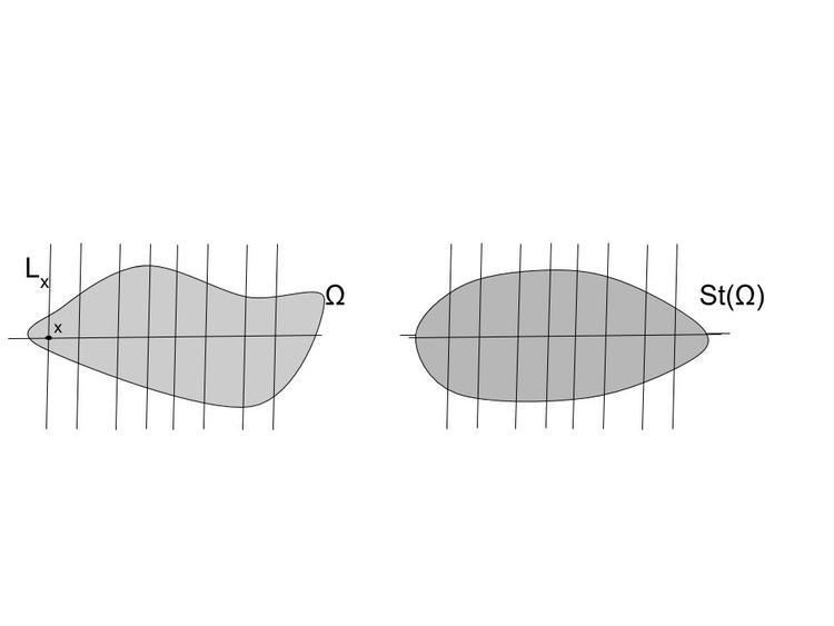
Steiner symmetrization was introduced by Steiner (1838) to solve the isoperimetric theorem stated above. Let H n − 1 ⊂ R n be a hyperplane through the origin. Rotate space so that H n − 1 is the x n = 0 hyperplane. For each x ∈ H let the perpendicular line through x ∈ H be L x = { x + y e n : y ∈ R } . Then by replacing each Ω ∩ L x by a line centered at H and with length | Ω ∩ L x | we obtain the Steiner symmetrized version.
St ( Ω ) := { x + y e n : x + z e n ∈ Ω for some z and | y | ≤ 1 2 | Ω ∩ L x | } . It is denoted by St ( f ) the Steiner symmetrization wrt to x n = 0 hyperplane of nonnegative measurable function f : R d → R and for fixed x 1 , … , x n − 1 define it as
S t : f ( x 1 , … , x n − 1 , ⋅ ) ↦ ( f ( x 1 , … , x n − 1 , ⋅ ) ) ∗ . A popular method for symmetrization in the plane is Polya's circular symmetrization. After, its generalization will be described to higher dimensions. Let Ω ⊂ C be a domain; then its circular symmetrization Circ ( Ω ) with regards to the positive real axis is defined as follows: Let
Ω t := { θ ∈ [ 0 , 2 π ] : t e i θ ∈ Ω }
i.e. contain the arcs of radius t contained in Ω . So it is defined
If Ω t is the full circle, then Circ ( Ω ) ∩ { | z | = t } := { | z | = t } .If the length is m ( Ω t ) = α , then Circ ( Ω ) ∩ { | z | = t } := { t e i θ : | θ | < α 2 } . 0 , ∞ ∈ Circ ( Ω ) iff 0 , ∞ ∈ Ω .In higher dimensions Ω ⊂ R n , its spherical symmetrization S p n ( Ω ) wrt to positive axis of x 1 is defined as follows: Let Ω r := { x ∈ S n − 1 : r x ∈ Ω } i.e. contain the caps of radius r contained in Ω . Also, for the first coordinate let angle ( x 1 ) := θ if x 1 = r c o s θ . So as above
If Ω r is the full cap, then S p n ( Ω ) ∩ { | z | = r } := { | z | = r } .If the surface area is m s ( Ω t ) = α , then S p n ( Ω ) ∩ { | z | = r } := { x : | x | = r and 0 ≤ angle ( x 1 ) ≤ θ α } =: C ( θ α ) where θ α is picked so that its surface area is m s ( C ( θ α ) = α . In words, C ( θ α ) is a cap symmetric around the positive axis x 1 with the same area as the intersection Ω ∩ { | z | = r } . 0 , ∞ ∈ S p n ( Ω ) iff 0 , ∞ ∈ Ω .Let Ω ⊂ R n be a domain and H n − 1 ⊂ R n be a hyperplane through the origin. Denote the reflection across that plane to the positive halfspace H + as σ H or just σ when it is clear from the context. Also, the reflected Ω across hyperplane H is defined as σ Ω . Then, the polarized Ω is denoted as Ω σ and defined as follows
If x ∈ Ω ∩ H + , then x ∈ Ω σ .If x ∈ Ω ∩ σ ( Ω ) ∩ H − , then x ∈ Ω σ .If x ∈ ( Ω ∖ σ ( Ω ) ) ∩ H − , then σ x ∈ Ω σ .In words, ( Ω ∖ σ ( Ω ) ) ∩ H − is simply reflected to the halfspace H + . It turns out that this transformation can approximate the above ones (in the Hausdorff distance) (see Brock & Solynin (2000)).