State observer

Discrete-time case

The state of a linear, time-invariant physical discrete-time system is assumed to satisfy

x ( k + 1 ) = A x ( k ) + B u ( k ) y ( k ) = C x ( k ) + D u ( k )

where, at time k , x ( k ) is the plant's state; u ( k ) is its inputs; and y ( k ) is its outputs. These equations simply say that the plant's current outputs and its future state are both determined solely by its current states and the current inputs. (Although these equations are expressed in terms of discrete time steps, very similar equations hold for continuous systems). If this system is observable then the output of the plant, y ( k ) , can be used to steer the state of the state observer.

The observer model of the physical system is then typically derived from the above equations. Additional terms may be included in order to ensure that, on receiving successive measured values of the plant's inputs and outputs, the model's state converges to that of the plant. In particular, the output of the observer may be subtracted from the output of the plant and then multiplied by a matrix L ; this is then added to the equations for the state of the observer to produce a so-called Luenberger observer, defined by the equations below. Note that the variables of a state observer are commonly denoted by a "hat": x ^ ( k ) and y ^ ( k ) to distinguish them from the variables of the equations satisfied by the physical system.

x ^ ( k + 1 ) = A x ^ ( k ) + L [ y ( k ) − y ^ ( k ) ] + B u ( k ) y ^ ( k ) = C x ^ ( k ) + D u ( k )

The observer is called asymptotically stable if the observer error e ( k ) = x ^ ( k ) − x ( k ) converges to zero when k → ∞ . For a Luenberger observer, the observer error satisfies e ( k + 1 ) = ( A − L C ) e ( k ) . The Luenberger observer for this discrete-time system is therefore asymptotically stable when the matrix A − L C has all the eigenvalues inside the unit circle.

For control purposes the output of the observer system is fed back to the input of both the observer and the plant through the gains matrix K .

u ( k ) = − K x ^ ( k )

The observer equations then become:

x ^ ( k + 1 ) = A x ^ ( k ) + L ( y ( k ) − y ^ ( k ) ) − B K x ^ ( k ) y ^ ( k ) = C x ^ ( k ) − D K x ^ ( k )

or, more simply,

x ^ ( k + 1 ) = ( A − B K ) x ^ ( k ) + L ( y ( k ) − y ^ ( k ) ) y ^ ( k ) = ( C − D K ) x ^ ( k )

Due to the separation principle we know that we can choose K and L independently without harm to the overall stability of the systems. As a rule of thumb, the poles of the observer A − L C are usually chosen to converge 10 times faster than the poles of the system A − B K .

Continuous-time case

The previous example was for an observer implemented in a discrete-time LTI system. However, the process is similar for the continuous-time case; the observer gains L are chosen to make the continuous-time error dynamics converge to zero asymptotically (i.e., when A − L C is a Hurwitz matrix).

For a continuous-time linear system

x ˙ = A x + B u , y = C x + D u ,

where x ∈ R n , u ∈ R m , y ∈ R r , the observer looks similar to discrete-time case described above:

x ^ ˙ = A x ^ + B u + L ( y − y ^ ) . y ^ = C x ^ + D u ,

The observer error e = x − x ^ satisfies the equation

e ˙ = ( A − L C ) e .

The eigenvalues of the matrix A − L C can be made arbitrarily by appropriate choice of the observer gain L when the pair [ A , C ] is observable, i.e. observability condition holds. In particular, it can be made Hurwitz, so the observer error e ( t ) → 0 when t → ∞ .

Peaking and other observer methods

When the observer gain L is high, the linear Luenberger observer converges to the system states very quickly. However, high observer gain leads to a peaking phenomenon in which initial estimator error can be prohibitively large (i.e., impractical or unsafe to use). As a consequence, nonlinear high gain observer methods are available that converge quickly without the peaking phenomenon. For example, sliding mode control can be used to design an observer that brings one estimated state's error to zero in finite time even in the presence of measurement error; the other states have error that behaves similarly to the error in a Luenberger observer after peaking has subsided. Sliding mode observers also have attractive noise resilience properties that are similar to a Kalman filter. Another approach is to apply multi observer, that significantly improves transients and reduces observer overshoot. Multi observer can be adapted to every system where High Gain Observer is applicable.

State observers for nonlinear systems

Sliding mode observers can be designed for the non-linear systems as well. For simplicity, first consider the no-input non-linear system:

x ˙ = f ( x )

where x ∈ R n . Also assume that there is a measurable output y ∈ R given by

y = h ( x ) .

There are several non-approximate approaches for designing an observer. The two observers given below also apply to the case when the system has an input. That is,

x ˙ = f ( x ) + B ( x ) u , y = h ( x ) , .

Linearizable error dynamics

One suggestion by Krener and Isidori and Krener and Respondek can be applied in a situation when there exists a linearizing transformation (i.e., a diffeomorphism, like the one used in feedback linearization) z = Φ ( x ) such that in new variables the system equations read

z ˙ = A z + ϕ ( y ) , y = C z .

The Luenberger observer is then designed as

z ^ ˙ = A z ^ + ϕ ( y ) − L ( C z ^ − y ) .

The observer error for the transformed variable e = z ^ − z satisfies the same equation as in classical linear case.

e ˙ = ( A − L C ) e .

As shown by Gauthier, Hammouri, and Othman and Hammouri and Kinnaert, if there exists transformation z = Φ ( x ) such that the system can be transformed into the form

z ˙ = A ( u ( t ) ) z + ϕ ( y , u ( t ) ) , y = C z ,

then the observer is designed as

z ^ ˙ = A ( u ( t ) ) z ^ + ϕ ( y , u ( t ) ) − L ( t ) ( C z ^ − y ) ,

where L ( t ) is a time-varying observer gain.

Ciccarella, Dalla Mora, and Germani obtained more advanced and general results, removing the need for a nonlinear transform and proving global asymptotic convergence of the estimated state to the true state using only simple assumptions on regularity.

Sliding mode observer

As discussed for the linear case above, the peaking phenomenon present in Luenberger observers justifies the use of a sliding mode observer. The sliding mode observer uses non-linear high-gain feedback to drive estimated states to a hypersurface where there is no difference between the estimated output and the measured output. The non-linear gain used in the observer is typically implemented with a scaled switching function, like the signum (i.e., sgn) of the estimated – measured output error. Hence, due to this high-gain feedback, the vector field of the observer has a crease in it so that observer trajectories slide along a curve where the estimated output matches the measured output exactly. So, if the system is observable from its output, the observer states will all be driven to the actual system states. Additionally, by using the sign of the error to drive the sliding mode observer, the observer trajectories become insensitive to many forms of noise. Hence, some sliding mode observers have attractive properties similar to the Kalman filter but with simpler implementation.

As suggested by Drakunov, a sliding mode observer can also be designed for a class of non-linear systems. Such an observer can be written in terms of original variable estimate x ^ and has the form

x ^ ˙ = [ ∂ H ( x ^ ) ∂ x ] − 1 M ( x ^ ) sgn ⁡ ( V ( t ) − H ( x ^ ) )

where:

The sgn ⁡ ( ⋅ ) vector extends the scalar signum function to n dimensions. That is,

for the vector z ∈ R n .

The vector H ( x ) has components that are the output function h ( x ) and its repeated Lie derivatives. In particular,

where L f i h is the i^th Lie derivative of output function h along the vector field f (i.e., along x trajectories of the non-linear system). In the special case where the system has no input or has a relative degree of n, H ( x ( t ) ) is a collection of the output y ( t ) = h ( x ( t ) ) and its n − 1 derivatives. Because the inverse of the Jacobian linearization of H ( x ) must exist for this observer to be well defined, the transformation H ( x ) is guaranteed to be a local diffeomorphism.

The diagonal matrix M ( x ^ ) of gains is such that

where, for each i ∈ { 1 , 2 , … , n } , element m i ( x ^ ) > 0 and suitably large to ensure reachability of the sliding mode.

The observer vector V ( t ) is such that

where sgn ⁡ ( ⋅ ) here is the normal signum function defined for scalars, and { … } eq denotes an "equivalent value operator" of a discontinuous function in sliding mode.

The idea can be briefly explained as follows. According to the theory of sliding modes, in order to describe the system behavior, once sliding mode starts, the function sgn ⁡ ( v i ( t ) − h i ( x ^ ( t ) ) ) should be replaced by equivalent values (see equivalent control in the theory of sliding modes). In practice, it switches (chatters) with high frequency with slow component being equal to the equivalent value. Applying appropriate lowpass filter to get rid of the high frequency component on can obtain the value of the equivalent control, which contains more information about the state of the estimated system. The observer described above uses this method several times to obtain the state of the nonlinear system ideally in finite time.

The modified observation error can be written in the transformed states e = H ( x ) − H ( x ^ ) . In particular,

{ e ˙ = d d ⁡ t H ( x ) − d d ⁡ t H ( x ^ ) = d d ⁡ t H ( x ) − M ( x ^ ) sgn ⁡ ( V ( t ) − H ( x ^ ( t ) ) ) ,

and so

{ [ e ˙ 1 e ˙ 2 ⋮ e ˙ i ⋮ e ˙ n − 1 e ˙ n ] = [ h ˙ 1 ( x ) h ˙ 2 ( x ) ⋮ h ˙ i ( x ) ⋮ h ˙ n − 1 ( x ) h ˙ n ( x ) ] ⏞ d d ⁡ t H ( x ) − M ( x ^ ) sgn ⁡ ( V ( t ) − H ( x ^ ( t ) ) ) ⏞ d d ⁡ t H ( x ^ ) = [ h 2 ( x ) h 3 ( x ) ⋮ h i + 1 ( x ) ⋮ h n ( x ) L f n h ( x ) ] − [ m 1 sgn ⁡ ( v 1 ( t ) − h 1 ( x ^ ( t ) ) ) m 2 sgn ⁡ ( v 2 ( t ) − h 2 ( x ^ ( t ) ) ) ⋮ m i sgn ⁡ ( v i ( t ) − h i ( x ^ ( t ) ) ) ⋮ m n − 1 sgn ⁡ ( v n − 1 ( t ) − h n − 1 ( x ^ ( t ) ) ) m n sgn ⁡ ( v n ( t ) − h n ( x ^ ( t ) ) ) ] = [ h 2 ( x ) − m 1 ( x ^ ) sgn ⁡ ( v 1 ( t ) ⏞ v 1 ( t ) = y ( t ) = h 1 ( x ) − h 1 ( x ^ ( t ) ) ⏞ e 1 ) h 3 ( x ) − m 2 ( x ^ ) sgn ⁡ ( v 2 ( t ) − h 2 ( x ^ ( t ) ) ) ⋮ h i + 1 ( x ) − m i ( x ^ ) sgn ⁡ ( v i ( t ) − h i ( x ^ ( t ) ) ) ⋮ h n ( x ) − m n − 1 ( x ^ ) sgn ⁡ ( v n − 1 ( t ) − h n − 1 ( x ^ ( t ) ) ) L f n h ( x ) − m n ( x ^ ) sgn ⁡ ( v n ( t ) − h n ( x ^ ( t ) ) ) ] .

So:

1. As long as m 1 ( x ^ ) ≥ | h 2 ( x ( t ) ) | , the first row of the error dynamics, e ˙ 1 = h 2 ( x ^ ) − m 1 ( x ^ ) sgn ⁡ ( e 1 ) , will meet sufficient conditions to enter the e 1 = 0 sliding mode in finite time.
2. Along the e 1 = 0 surface, the corresponding v 2 ( t ) = { m 1 ( x ^ ) sgn ⁡ ( e 1 ) } eq equivalent control will be equal to h 2 ( x ) , and so v 2 ( t ) − h 2 ( x ^ ) = h 2 ( x ) − h 2 ( x ^ ) = e 2 . Hence, so long as m 2 ( x ^ ) ≥ | h 3 ( x ( t ) ) | , the second row of the error dynamics, e ˙ 2 = h 3 ( x ^ ) − m 2 ( x ^ ) sgn ⁡ ( e 2 ) , will enter the e 2 = 0 sliding mode in finite time.
3. Along the e i = 0 surface, the corresponding v i + 1 ( t ) = { … } eq equivalent control will be equal to h i + 1 ( x ) . Hence, so long as m i + 1 ( x ^ ) ≥ | h i + 2 ( x ( t ) ) | , the ( i + 1 ) ^th row of the error dynamics, e ˙ i + 1 = h i + 2 ( x ^ ) − m i + 1 ( x ^ ) sgn ⁡ ( e i + 1 ) , will enter the e i + 1 = 0 sliding mode in finite time.

So, for sufficiently large m i gains, all observer estimated states reach the actual states in finite time. In fact, increasing m i allows for convergence in any desired finite time so long as each | h i ( x ( 0 ) ) | function can be bounded with certainty. Hence, the requirement that the map H : R n → R n is a diffeomorphism (i.e., that its Jacobian linearization is invertible) asserts that convergence of the estimated output implies convergence of the estimated state. That is, the requirement is an observability condition.

In the case of the sliding mode observer for the system with the input, additional conditions are needed for the observation error to be independent of the input. For example, that

∂ H ( x ) ∂ x B ( x )

does not depend on time. The observer is then

x ^ ˙ = [ ∂ H ( x ^ ) ∂ x ] − 1 M ( x ^ ) sgn ⁡ ( V ( t ) − H ( x ^ ) ) + B ( x ^ ) u .

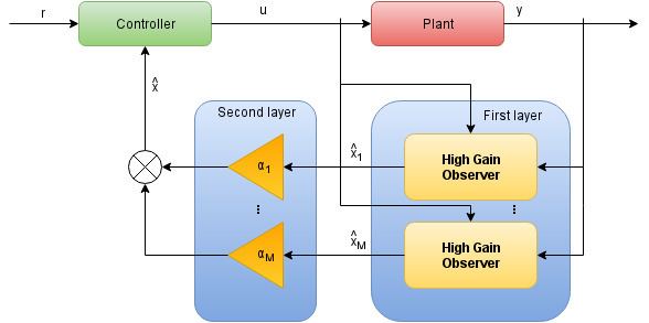
Multi Observer

Multi observer extends High Gain Observer structure from single to multi observer, with many models working simultaneously. This has two layers: the first consists of multiple High Gain Observers with different estimation states, and the second determines the importance weights of the first layer observers. The algorithm is simple to implement and does not contain any risky operations like differentiation. The idea of multiple models was previously applied to obtain information in adaptive control .

Assume that the number of High Gain Observers equals n+1

x k ^ ˙ ( t ) = A x k ^ ( t ) + B ϕ 0 ( x ^ ( t ) , u ( t ) ) − L ( y k ^ ( t ) − y ( t ) ) y k ^ ( t ) = C x k ^ ( t )

where k = 1... n + 1 is the observer index. The first layer observers consists of the same gain L but they differ with the initial state x k ( 0 ) . In the second layer all x k ( t ) from k = 1... n + 1 observers are combined into one to obtain single state vector estimation

y k ^ ( t ) = ∑ k = 1 n + 1 α k ( t ) x k ^ ( t )

where α k ∈ R are weight factors. These factors are changed to provide the estimation in the second layer and to improve the observation process.

Let assume that

∑ k = 1 n + 1 α k ( t ) ξ k ( t ) = 0

and

∑ k = 1 n + 1 α k ( t ) = 1

where ξ k ∈ R n × 1 is some vector that depends on k t h observer error e k ( t ) .

Some transformation yields to linear regression problem

[ − ξ n + 1 ( t ) ] = [ ξ 1 ( t ) − ξ n + 1 ( t ) … ξ k ( t ) − ξ n + 1 ( t ) … ξ n ( t ) − ξ n + 1 ( t ) ] T [ α 1 ( t ) ⋮ α k ( t ) ⋮ α n ( t ) ]

This formula gives possibility to estimate α k ( t ) . To construct mainfold we need mapping m : R n → R n between ξ k ( t ) = m ( e k ( t ) ) and ensurance that ξ k ( t ) is calculable relying on measurable signals. First thing is to eliminate paeking phenomenon for α k ( t ) from observer error

e σ ( t ) = ∑ k = 1 n + 1 α k ( t ) e k ( t ) .

Calculate n times derivative on η k ( t ) = y ^ k ( t ) − y ( t ) to find mapping m lead to ξ k ( t ) defined as

ξ k ( t ) = [ 1 0 0 ⋯ 0 C L 1 0 ⋯ 0 C A L C L 1 ⋯ 0 C A 2 L C A L C L ⋯ 0 ⋮ ⋮ ⋮ ⋱ C A n − 2 L C A n − 3 L C A n − 4 L ⋯ 1 ] [ ∫ t − t d t n − 1 ⋯ ∫ t − t d t η k ( τ ) d τ ⋮ η ( t ) − η ( t − ( n − 1 ) t d ) ]

where t d > 0 is some time constant. Note that ξ k ( t ) relays on both η k ( t ) and its integrals hence it is easily available in the control system. Further α k ( t ) is specified by estimation law; and thus it proves that mainfold is measurable. In the second layer α ^ k ( t ) for k = 1 … n + 1 is introduced as estimates of α k ( t ) coefficients. The mapping error is specified as

e ξ ( t ) = ∑ k = 1 n + 1 α ^ k ( t ) ξ k ( t )

where e ξ ( t ) ∈ R n × 1 , α ^ k ( t ) ∈ R . If coefficients α ^ ( t ) are equal to α k ( t ) , then mapping error e ξ ( t ) = 0 Now it is possible to calculate x ^ from above equation and hence the peaking phenomenon is reduced thanks to properties of mainfold. The created mapping gives a lot of flexibility in the estimation process. Even it is possible to estimate the value of x ( t ) in the second layer and to calculate the state x .

Bounding observers

The Bounding or Interval observers constitute a class of observers that provide two estimations of the state simultaneously: one of the estimations provides an upper bound on the real value of the state, whereas the second one provides a lower bound. The real value of the state is then known to be always within these two estimations.

These bounds are very important in practical applications, as they make possible to know at each time the precision of the estimation.

Mathematically, two Luenberger observers can be used, if L is properly selected, using, for example, positive systems properties: one for the upper bound x ^ U ( k ) (that ensures that e ( k ) = x ^ U ( k ) − x ( k ) converges to zero from above when k → ∞ , in the absence of noise and uncertainty), and a lower bound x ^ L ( k ) (that ensures that e ( k ) = x ^ L ( k ) − x ( k ) converges to zero from below). That is, always x ^ U ( k ) ≥ x ( k ) ≥ x ^ L ( k )