The squirmer is a model for a spherical microswimmer swimming in Stokes flow. The squirmer model was introduced by James Lighthill in 1952 and refined and used to model Paramecium by John Blake in 1971. Blake used the squirmer model to describe the flow generated by a carpet of beating short filaments called cilia on the surface of Paramecium. Today, the squirmer is a standard model for the study of self-propelled particles, such as Janus particles, in Stokes flow.
Velocity field in particle frame
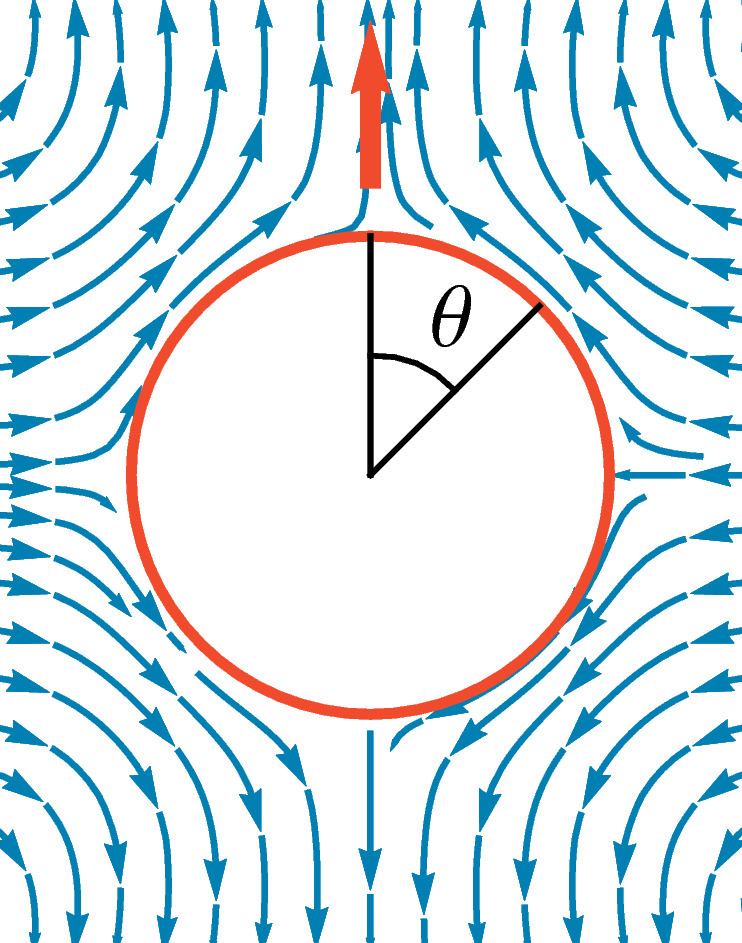
Here we give the flow field of a squirmer in the case of a non-deformable axisymmetric spherical squirmer (radius R ). These expressions are given in a spherical coordinate system.
u r ( r , θ ) = 2 3 ( R 3 r 3 − 1 ) B 1 P 1 ( cos θ ) + ∑ n = 2 ∞ ( R n + 2 r n + 2 − R n r n ) B n P n ( cos θ ) ,
u θ ( r , θ ) = 2 3 ( R 3 2 r 3 + 1 ) B 1 V 1 ( cos θ ) + ∑ n = 2 ∞ 1 2 ( n R n + 2 r n + 2 + ( 2 − n ) R n r n ) B n V n ( cos θ ) .
Here B n are constant coefficients, P n ( cos θ ) are Legendre polynomials, and V n ( cos θ ) = − 2 n ( n + 1 ) ∂ θ P n ( cos θ ) .
One finds P 1 ( cos θ ) = cos θ , P 2 ( cos θ ) = 1 2 ( 3 cos 2 θ − 1 ) , … , V 1 ( cos θ ) = sin θ , V 2 ( cos θ ) = 1 2 sin 2 θ , … .
The expressions above are in the frame of the moving particle. At the interface one finds u θ ( R , θ ) = ∑ n = 1 ∞ B n V n and u r ( R , θ ) = 0 .
Swimming speed and lab frame
By using the Lorentz Reciprocal Theorem, one finds the velocity vector of the particle U = − 1 2 ∫ u ( R , θ ) sin θ d θ = 2 3 B 1 e z . The flow in a fixed lab frame is given by u L = u + U :
u r L ( r , θ ) = R 3 r 3 U P 1 ( cos θ ) + ∑ n = 2 ∞ ( R n + 2 r n + 2 − R n r n ) B n P n ( cos θ ) ,
u θ L ( r , θ ) = R 3 2 r 3 U V 1 ( cos θ ) + ∑ n = 2 ∞ 1 2 ( n R n + 2 r n + 2 + ( 2 − n ) R n r n ) B n V n ( cos θ ) .
with swimming speed U = | U | . Note, that lim r → ∞ u L = 0 and u r L ( R , θ ) ≠ 0 .
Structure of the flow and squirmer parameter
The series above are often truncated at n = 2 in the study of far field flow, r ≫ R . Within that approximation, u θ ( R , θ ) = B 1 sin θ + 1 2 B 2 sin 2 θ , with squirmer parameter β = B 2 / | B 1 | . The first mode n = 1 characterizes a hydrodynamic source dipole with decay ∝ 1 / r 3 (and with that the swimming speed U ). The second mode n = 2 corresponds to a hydrodynamic stresslet or force dipole with decay ∝ 1 / r 2 . Thus, β gives the ratio of both contributions and the direction of the force dipole. β is used to categorize microswimmers into pushers, pullers and neutral swimmers.
As can be seen in the figures above, the (lab frame) velocity field of the passive particle corresponds to a monopole. Furthermore, the B 1 mode corresponds to a dipole (see case β = 0 ) and the B 2 mode corresponds to a quadrupole (see cases β ≠ 0 ).