Split complex number

Definition

A split-complex number is an ordered pair of real numbers, written in the form

where x and y are real numbers and the quantity j satisfies

Choosing j 2 = − 1 results in the complex numbers. It is this sign change which distinguishes the split-complex numbers from the ordinary complex ones. The quantity j here is not a real number but an independent quantity; that is, it is not equal to ±1.

The collection of all such z is called the split-complex plane. Addition and multiplication of split-complex numbers are defined by

This multiplication is commutative, associative and distributes over addition.

Conjugate, modulus, and bilinear form

Just as for complex numbers, one can define the notion of a split-complex conjugate. If

the conjugate of z is defined as

The conjugate satisfies similar properties to usual complex conjugate. Namely,

These three properties imply that the split-complex conjugate is an automorphism of order 2.

The modulus of a split-complex number z = x + j y is given by the isotropic quadratic form

It has the composition algebra property:

However, this quadratic form is not positive-definite but rather has signature (1, −1), so the modulus is not a norm.

The associated bilinear form is given by

where z = x + j y and w = u + j v. Another expression for the modulus is then

Since it is not positive-definite, this bilinear form is not an inner product; nevertheless the bilinear form is frequently referred to as an indefinite inner product. A similar abuse of language refers to the modulus as a norm.

A split-complex number is invertible if and only if its modulus is nonzero ( ∥ z ∥ ≠ 0 ), thus x ± j x have no inverse. The multiplicative inverse of an invertible element is given by

Split-complex numbers which are not invertible are called null vectors. These are all of the form (a ± j a) for some real number a.

The diagonal basis

There are two nontrivial idempotent elements given by e = (1 − j)/2 and e^∗ = (1 + j)/2. Recall that idempotent means that ee = e and e^∗e^∗ = e^∗. Both of these elements are null:

It is often convenient to use e and e^∗ as an alternate basis for the split-complex plane. This basis is called the diagonal basis or null basis. The split-complex number z can be written in the null basis as

If we denote the number z = ae + be^∗ for real numbers a and b by (a, b), then split-complex multiplication is given by

In this basis, it becomes clear that the split-complex numbers are ring-isomorphic to the direct sum R ⊕ R with addition and multiplication defined pairwise.

The split-complex conjugate in the diagonal basis is given by

and the modulus by

Though lying in the same isomorphism class in the category of rings, the split-complex plane and the direct sum of two real lines differ in their layout in the Cartesian plane. The isomorphism, as a planar mapping, consists of a counter-clockwise rotation by 45° and a dilation by √2. The dilation in particular has sometimes caused confusion in connection with areas of hyperbolic sectors. Indeed, hyperbolic angle corresponds to area of sectors in the R ⊕ R plane with its "unit circle" given by { ( a , b ) ∈ R ⊕ R : a b = 1 } . The contracted "unit circle" { cosh ⁡ a + j   sinh ⁡ a : a ∈ R } of the split-complex plane has only half the area in the span of a corresponding hyperbolic sector. Such confusion may be perpetuated when the geometry of the split-complex plane is not distinguished from that of R ⊕ R .

Geometry

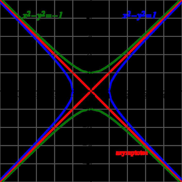
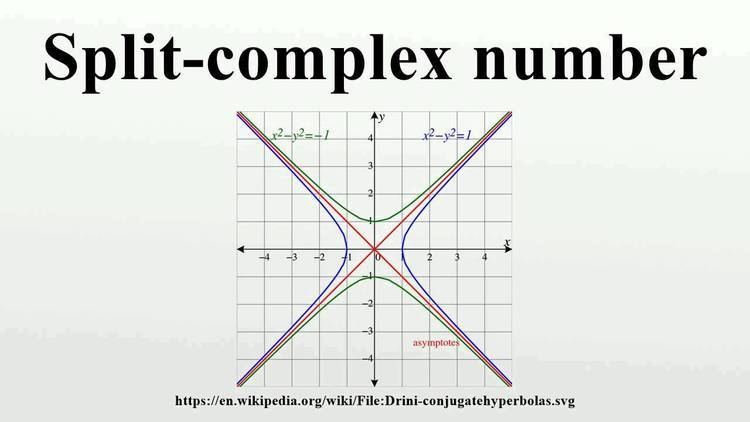
A two-dimensional real vector space with the Minkowski inner product is called (1 + 1)-dimensional Minkowski space, often denoted R^1,1. Just as much of the geometry of the Euclidean plane R² can be described with complex numbers, the geometry of the Minkowski plane R^1,1 can be described with split-complex numbers.

The set of points

is a hyperbola for every nonzero a in R. The hyperbola consists of a right and left branch passing through (a, 0) and (−a, 0). The case a = 1 is called the unit hyperbola. The conjugate hyperbola is given by

with an upper and lower branch passing through (0, a) and (0, −a). The hyperbola and conjugate hyperbola are separated by two diagonal asymptotes which form the set of null elements:

These two lines (sometimes called the null cone) are perpendicular in R² and have slopes ±1.

Split-complex numbers z and w are said to be hyperbolic-orthogonal if ⟨z, w⟩ = 0. While analogous to ordinary orthogonality, particularly as it is known with ordinary complex number arithmetic, this condition is more subtle. It forms the basis for the simultaneous hyperplane concept in spacetime.

The analogue of Euler's formula for the split-complex numbers is

This can be derived from a power series expansion using the fact that cosh has only even powers while that for sinh has odd powers. For all real values of the hyperbolic angle θ the split-complex number λ = exp(jθ) has norm 1 and lies on the right branch of the unit hyperbola. Numbers such as λ have been called hyperbolic versors.

Since λ has modulus 1, multiplying any split-complex number z by λ preserves the modulus of z and represents a hyperbolic rotation (also called a Lorentz boost or a squeeze mapping). Multiplying by λ preserves the geometric structure, taking hyperbolas to themselves and the null cone to itself.

The set of all transformations of the split-complex plane which preserve the modulus (or equivalently, the inner product) forms a group called the generalized orthogonal group O(1, 1). This group consists of the hyperbolic rotations, which form a subgroup denoted SO⁺(1, 1), combined with four discrete reflections given by

The exponential map

sending θ to rotation by exp(jθ) is a group isomorphism since the usual exponential formula applies:

If a split-complex number z does not lie on one of the diagonals, then z has a polar decomposition.

Algebraic properties

In abstract algebra terms, the split-complex numbers can be described as the quotient of the polynomial ring R[x] by the ideal generated by the polynomial x² − 1,

The image of x in the quotient is the "imaginary" unit j. With this description, it is clear that the split-complex numbers form a commutative ring with characteristic 0. Moreover if we define scalar multiplication in the obvious manner, the split-complex numbers actually form a commutative and associative algebra over the reals of dimension two. The algebra is not a division algebra or field since the null elements are not invertible. In fact, all of the nonzero null elements are zero divisors. Since addition and multiplication are continuous operations with respect to the usual topology of the plane, the split-complex numbers form a topological ring.

The algebra of split-complex numbers forms a composition algebra since

The class of composition algebras extends the normed algebras class which also has this composition property.

From the definition it is apparent that the ring of split-complex numbers is isomorphic to the group ring R[C₂] of the cyclic group C₂ over the real numbers R.

Matrix representations

One can easily represent split-complex numbers by matrices. The split-complex number

can be represented by the matrix

Addition and multiplication of split-complex numbers are then given by matrix addition and multiplication. The modulus of z is given by the determinant of the corresponding matrix. In this representation, split-complex conjugation corresponds to multiplying on both sides by the matrix

For any real number a, a hyperbolic rotation by a hyperbolic angle a corresponds to multiplication by the matrix

The diagonal basis for the split-complex number plane can be invoked by using an ordered pair (x, y) for z = x + j y and making the mapping

Now the quadratic form is u v = ( x + y ) ( x − y ) = x 2 − y 2 . Furthermore,

so the two parametrized hyperbolas are brought into correspondence with S. The action of hyperbolic versor e b j then corresponds under this linear transformation to a squeeze mapping

Note that in the context of 2 × 2 real matrices there are in fact a great number of different representations of split-complex numbers. The above diagonal representation represents the Jordan canonical form of the matrix representation of the split-complex numbers. For a split-complex number z = (x, y) given by the following matrix representation:

Its Jordan canonical form is given by:

where Z = S J z S − 1   , and

History

The use of split-complex numbers dates back to 1848 when James Cockle revealed his tessarines. William Kingdon Clifford used split-complex numbers to represent sums of spins. Clifford introduced the use of split-complex numbers as coefficients in a quaternion algebra now called split-biquaternions. He called its elements "motors", a term in parallel with the "rotor" action of an ordinary complex number taken from the circle group. Extending the analogy, functions of a motor variable contrast to functions of an ordinary complex variable.

Since the early twentieth century, the split-complex multiplication has commonly been seen as a Lorentz boost of a spacetime plane. In that model, the number z = x + y j represents an event in a spacio-temporal plane, where x is measured in nanoseconds and y in Mermin’s feet. The future corresponds to the quadrant of events {z : | y | < x }, which has the split-complex polar decomposition z = ρ e a j . The model says that z can be reached from the origin by entering a frame of reference of rapidity a and waiting ρ nanoseconds. The split-complex equation

expressing products on the unit hyperbola illustrates the additivity of rapidities for collinear velocities. Simultaneity of events depends on rapidity a;

is the line of events simultaneous with the origin in the frame of reference with rapidity a. Two events z and w are hyperbolic-orthogonal when z^∗w + zw^∗ = 0. Canonical events exp(aj) and j exp(aj) are hyperbolic orthogonal and lie on the axes of a frame of reference in which the events simultaneous with the origin are proportional to j exp(aj).

In 1933 Max Zorn was using the split-octonions and noted the composition algebra property. He realized that the Cayley–Dickson construction, used to generate division algebras, could be modified (with a factor gamma (γ)) to construct other composition algebras including the split-octonions. His innovation was perpetuated by Adrian Albert, Richard D. Schafer, and others. The gamma factor, with ℝ as base field, builds split-complex numbers as a composition algebra. Reviewing Albert for Mathematical Reviews, N. H. McCoy wrote that there was an "introduction of some new algebras of order 2^e over F generalizing Cayley–Dickson algebras." Taking F = ℝ and e = 1 corresponds to the algebra of this article.

In 1935 J.C. Vignaux and A. Durañona y Vedia developed the split-complex geometric algebra and function theory in four articles in Contribución a las Ciencias Físicas y Matemáticas, National University of La Plata, República Argentina (in Spanish). These expository and pedagogical essays presented the subject for broad appreciation.

In 1941 E.F. Allen used the split-complex geometric arithmetic to establish the nine-point hyperbola of a triangle inscribed in zz^∗ = 1.

In 1956 Mieczyslaw Warmus published "Calculus of Approximations" in Bulletin de l’Academie Polanaise des Sciences (see link in References). He developed two algebraic systems, each of which he called "approximate numbers", the second of which forms a real algebra. D. H. Lehmer reviewed the article in Mathematical Reviews and observed that this second system was isomorphic to the "hyperbolic complex" numbers, the subject of this article.

In 1961 Warmus continued his exposition, referring to the components of an approximate number as midpoint and radius of the interval denoted.

Synonyms

Different authors have used a great variety of names for the split-complex numbers. Some of these include:

Split-complex numbers and their higher-dimensional relatives (split-quaternions / coquaternions and split-octonions) were at times referred to as "Musean numbers", since they are a subset of the hypernumber program developed by Charles Musès.