Spacetime triangle diagram technique - Alchetron, the free social encyclopedia

In physics and mathematics, the spacetime triangle diagram (STTD) technique, also known as the Smirnov method of incomplete separation of variables, is the direct space-time domain method for electromagnetic and scalar wave motion.

Basic stages

(Electromagnetics) The system of Maxwell's equations is reduced to a second-order PDE for the field components, or potentials, or their derivatives.
The spatial variables are separated using convenient expansions into series and/or integral transforms—except one that remains bounded with the time variable, resulting in a PDE of hyperbolic type.
The resulting hyperbolic PDE and the simultaneously transformed initial conditions compose a problem, which is solved using the Riemann–Volterra integral formula. This yields the generic solution expressed via a double integral over a triangle domain in the bounded-coordinate—time space. Then this domain is replaced by a more complicated but smaller one, in which the integrant is essentially nonzero, found using a strictly formalized procedure involving specific spacetime triangle diagrams (see, e.g., Refs.).
In the majority of cases the obtained solutions, being multiplied by known functions of the previously separated variables, result in the expressions of a clear physical meaning (nonsteady-state modes). In many cases, however, more explicit solutions can be found summing up the expansions or doing the inverse integral transform.

STTD versus Green's function technique

The STTD technique belongs to the second among the two principal ansätze for theoretical treatment of waves — the frequency domain and the direct spacetime domain. The most well-established method for the inhomogeneous (source-related) descriptive equations of wave motion is one based on the Green's function technique. For the circumstances described in Section 6.4 and Chapter 14 of Jackson's Classical Electrodynamics, it can be reduced to calculation of the wave ﬁeld via retarded potentials (in particular, the Liénard–Wiechert potentials).

Despite certain similarity between Green's and Riemann–Volterra methods (in some literature the Riemann function is called the Riemann–Green function ), their application to the problems of wave motion results in distinct situations:

The definitions of both Green's function and corresponding Green's solution are not unique as they leave room for addition of arbitrary solution of the homogeneous equation; in some circumstances the particular choice of Green's function and the final solution are defined by boundary condition(s) or plausibility and physical admissibility of the constructed wavefunctions. The Riemann function is a solution of the homogeneous equation that additionally must take a certain value at the characteristics and thus is defined in a unique way.

In contrast to Green's method that provides a particular solution of the inhomogeneous equation, the Riemann–Volterra method is related to the corresponding problem, comprising the PDE and initial conditions,

and it was the Riemann–Volterra representation that Smirnov used in his Course of Higher Mathematics to prove the uniqueness of the solution to the above problem (see, item 143).

In the general case, Green's formula implies integration over the entire domain of variation of coordinates and time, while integration in the Riemann–Volterra solution is carried out within a limited triangle region, assuring the boundness of the solution support.

Causality of the (unique) Riemann–Volterra solution is provided automatically, without need to recur to additional considerations, such as the retarded nature of the argument, wave propagation in certain direction, specific choice of the integration path, etc. (Usually the descriptive equations, such as the classical scalar wave equation, possess the T-symmetry. It is the time-asymmetric initial conditions that define the arrow of time through the limitation of the integration domain in the Riemann formula to t > 0 , see more in and a particular example given below.)

Green's function can be readily derived from the Liénard–Wiechert potential of a moving point source, but concrete calculation of the wavefunction, inevitably involving the analysis of the retarded argument, may develop in a rather complicated task unless some special techniques, like the parametric method,

are invoked. The Riemann-Volterra approach presents the same or even more serious difficulties, especially when one deals with the bounded-support sources: here the actual limits of integration must be defined from the system of inequalities involving the space-time variables and parameters of the source term. However, this definition can be strictly formalized using the spacetime triangle diagrams. Playing the same role as the Feynman diagrams in particle physics, STTDs provide a strict and illustrative procedure for definition of areas with the same analytic representation of the integration domain in the 2D space spanned by the non-separated spatial variable and time.

Drawbacks of the method

The method can only be applied to problems possessing known Riemann function.

Application of the method and analysis of the results obtained require more profound knowledge of the special functions of mathematical physics (e.g., operating with the generalized functions, Mathieu functions of different kinds and Lommel’s functions of two variables) than Green's function method.

In some cases the final integrals require special consideration in the domains of rapid oscillation of the Riemann function.

General considerations

Several efficient methods for scalarizing electromagnetic problems in the orthogonal coordinates x 1 , x 2 , x 3 were discussed by Borisov in Ref. The most important conditions of their applicability are h 3 = 1 and ∂ 3 ( h 1 / h 2 ) = 0 , where h i , i = 1 , 2 , 3 are the metric (Lamé) coefficients (so that the squared length element is d s 2 = h 1 2 d x 1 2 + h 2 2 d x 2 2 + h 3 2 d x 3 2 ). Remarkably, this condition is met for the majority of practically important coordinate systems, including the Cartesian, general-type cylindrical and spherical ones.

For the problems of wave motion is free space, the basic method of separating spatial variables is the application of integral transforms, while for the problems of wave generation and propagation in the guiding systems the variables are usually separated using expansions in terms of the basic functions (modes) meeting the required boundary conditions at the surface of the guiding system.

Cartesian and cylindrical coordinates

In the Cartesian { x 1 = x , x 2 = y , x 3 = z } and general-type cylindrical coordinates { x 1 = x 1 ( x , y ) , x 2 = x 2 ( x , y ) , x 3 = z } separation of the spatial variables result in the initial value problem for a hyperbolic PDE known as the 1D Klein–Gordon equation (KGE)

( ∂ τ 2 − ∂ z 2 + k 2 ) ψ ( τ , z ) = f ( τ , z ) ψ ( τ , z ) = 0 for τ < 0

Here τ is the time variable expressed in units of length using some characteristic velocity (e.g., speed of light or sound), k is a constant originated from the separation of variables, and f ( τ , z ) represents a part of the source term in the initial wave equation that remains after application of the variable-separation procedures (a series coefficient or a result of an integral transform).

The above problem possesses known Riemann function

R k ( τ , z ; τ ′ , z ′ ) = J 0 ( k ( τ − τ ′ ) 2 − ( z − z ′ ) 2 ) ,

where J 0 ( ⋅ ) is the Bessel function of the first kind of order zero.

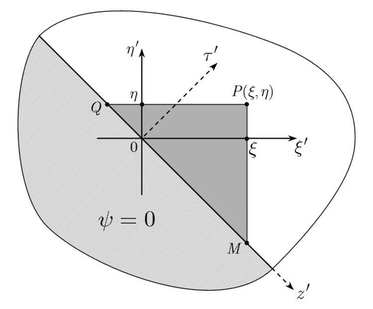
Passing to the canonical variables z , τ → ξ , η one gets the simplest STTD diagram reflecting straightforward application of the Riemann–Volterra method, with the fundamental integration domain represented by spacetime triangle MPQ (in dark grey).

Rotation of the STTD 45° counter clockwise yields more common form of the STTD in the conventional spacetime z , τ .

For the homogeneous initial conditions the (unique) solution of the problem is given by the Riemann formula

ψ ( τ , z ) = 1 2 ∬ △ M P Q d τ ′ d z ′ R ( τ , z ; τ ′ , z ′ ) f ( τ ′ , z ′ ) .

Evolution of the wave process can be traced using a fixed observation point ( z = const ) successively increasing the triangle height ( τ ) or, alternatively, taking "momentary picture" of the wavefunction ψ by shifting the spacetime triangle along the z axis ( τ = const ).

More useful and sophisticated STTDs correspond to pulsed sources whose support is limited in spacetime. Each limitation produce specific modifications in the STTD, resulting to smaller and more complicated integration domains in which the integrand is essentially non-zero. Examples of most common modifications and their combined actions are illustrated below.

Spherical coordinates

In the spherical coordinate system — which in view of the General considerations must be represented in the sequence { x 1 = θ , x 2 = φ , x 3 = r } , assuring h 3 = 1 — one can scalarize problems for the transverse electric (TE) or transverse magnetic (TM) waves using the Borgnis functions, Debye potentials or Hertz vectors. Subsequent separation of the angular variables θ , φ via expansion of the initial wavefunction ψ ( τ , θ , φ , r ) and the source

f ( τ , θ , φ , r ) in terms of ( sin ⁡ m φ cos ⁡ m φ ) P n ( m ) ( cos ⁡ θ ) ,

where P n ( m ) ( ⋅ ) is the associated Legendre polynomial of degree n and order m , results in the initial value problem for the hyperbolic Euler–Poisson–Darboux equation

( ∂ τ 2 − ∂ r 2 + n ( n + 1 ) r 2 ) ψ n m ( τ , r ) = f n m ( τ , r ) ψ n m ( τ , r ) = 0 for τ < 0

known to have the Riemann function

R ( τ , r ; τ ′ , r ′ ) = P n ( r 2 + r ′ 2 − ( τ − τ ′ ) 2 2 r r ′ ) ,

where P n ( ⋅ ) is the (ordinary) Legendre polynomial of degree n .

Equivalence of the STTD (Riemann) and Green's function solutions

The STTD technique represents an alternative to the classical Green's function method. Due to uniqueness of the solution to the initial value problem in question, in the particular case of zero initial conditions the Riemann solution provided by the STTD technique must coincide with the convolution of the causal Green’s function and the source term.

The two methods provide apparently different descriptions of the wavefunction: e.g., the Riemann function to the Klein–Gordon problem is a Bessel function (which must be integrated, together with the source term, over the restricted area represented by the fundamental triangle MPQ) while the retarded Green's function to the Klein–Gordon equation is a Fourier transform of the imaginary exponential term (to be integrated over the entire plane z ′ , τ ′ , see, for example, Sec. 3.1. of Ref. ) reducible to

G k ( τ , z ; τ ′ , z ′ ) = − 1 ( 2 π ) 2 ∫ − ∞ ∞ d p e i p ( z − z ′ ) ∫ − ∞ ∞ d Ω e i Ω ( τ − τ ′ ) Ω 2 − p 2 − k 2 .

Extending integration with respect to Ω to the complex domain, using the residue theorem (with the poles Ω 1 , 2 chosen as lim ε → 0 + ( ± p 2 + k 2 + i ε ) to satisfy the causality conditions) one gets

G k ( τ , z ; τ ′ , z ′ ) = 1 π ∫ 0 ∞ d p sin ⁡ ( ( τ − τ ′ ) p 2 + k 2 ) p 2 + k 2 cos ⁡ ( p ( z − z ′ ) ) .

Using formula 3.876-1 of Gradshteyn and Ryzhik,

∫ 0 ∞ d x sin ⁡ ( p x 2 + a 2 ) x 2 + a 2 cos ⁡ ( b x ) = { π 2 J 0 ( a p 2 − b 2 ) for 0 < b < p 0 for b > p > 0 ( a > 0 ) ,

the last Green's function representation reduces to the expression

1 2 J 0 ( k ( τ − τ ′ ) 2 − ( z − z ′ ) 2 ) h ( τ − τ ′ − | z − z ′ | ) ,

in which 1/2 is the scaling factor of the Riemann formula and J 0 ( ⋅ ) the Riemann function, while the Heaviside step function h ( ⋅ ) reduces, for τ > 0 , the area of integration to the fundamental triangle MPQ, making the Green's function solution equal to that provided by the STTD technique.

References

Spacetime triangle diagram technique Wikipedia

(Text) CC BY-SA

Contents