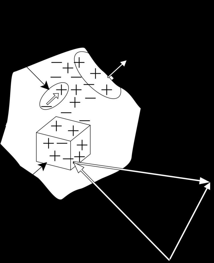
Retarded potential - Alchetron, The Free Social Encyclopedia

In electrodynamics, the retarded potentials are the electromagnetic potentials for the electromagnetic field generated by time-varying electric current or charge distributions in the past. The fields propagate at the speed of light c, so the delay of the fields connecting cause and effect at earlier and later times is an important factor: the signal takes a finite time to propagate from a point in the charge or current distribution (the point of cause) to another point in space (where the effect is measured), see figure below.

Potentials in the Lorentz gauge

The starting point is Maxwell's equations in the potential formulation using the Lorenz gauge:

◻ φ = − ρ ϵ 0 , ◻ A = − μ 0 J

where φ(r, t) is the electric potential and A(r, t) is the magnetic potential, for an arbitrary source of charge density ρ(r, t) and current density J(r, t), and ◻ is the D'Alembert operator. Solving these gives the retarded potentials below (all in SI units).

Retarded and advanced potentials for time-dependent fields

For time-dependent fields, the retarded potentials are:

φ ( r , t ) = 1 4 π ϵ 0 ∫ ρ ( r ′ , t r ) | r − r ′ | d 3 r ′ A ( r , t ) = μ 0 4 π ∫ J ( r ′ , t r ) | r − r ′ | d 3 r ′ .

where r is a point in space, t is time,

t r = t − | r − r ′ | c

is the retarded time, and d³r' is the integration measure using r'.

From φ(r,t) and A(r, t), the fields E(r, t) and B(r, t) can be calculated using the definitions of the potentials:

− E = ∇ φ + ∂ A ∂ t , B = ∇ × A .

and this leads to Jefimenko's equations. The corresponding advanced potentials have an identical form, except the advanced time

t a = t + | r − r ′ | c

replaces the retarded time.

Comparison with static potentials for time-independent fields

In the case the fields are time-independent (electrostatic and magnetostatic fields), the time derivatives in the ◻ operators of the fields are zero, and Maxwell's equations reduce to

∇ 2 φ = − ρ ϵ 0 , ∇ 2 A = − μ 0 J ,

where ∇² is the Laplacian, which take the form of Poisson's equation in four components (one for φ and three for A), and the solutions are:

φ ( r ) = 1 4 π ϵ 0 ∫ ρ ( r ′ ) | r − r ′ | d 3 r ′ A ( r ) = μ 0 4 π ∫ J ( r ′ ) | r − r ′ | d 3 r ′ .

These also follow directly from the retarded potentials.

Potentials in the Coulomb gauge

In the Coulomb gauge, Maxwell's equations are

∇ 2 φ = − ρ ϵ 0 ∇ 2 A − 1 c 2 ∂ 2 A ∂ t 2 = − μ 0 J + 1 c 2 ∇ ( ∂ φ ∂ t ) ,

although the solutions contrast the above, since A is a retarded potential yet φ changes instantly, given by:

φ ( r , t ) = 1 4 π ϵ 0 ∫ ρ ( r ′ , t ) | r − r ′ | d 3 r ′ A ( r , t ) = 1 4 π ε 0 ∇ × ∫ d 3 r ′ ∫ 0 | r − r ′ | / c d t r t r J ( r ′ , t − t r ) | r − r ′ | 3 × ( r − r ′ ) .

This presents an advantage and a disadvantage of the coulomb gauge - φ is easily calculable from the charge distribution ρ but A is not so easily calculable from the current distribution j. However, provided we require that the potentials vanish at infinity, they can be expressed neatly in terms of fields:

φ ( r , t ) = 1 4 π ∫ ∇ ⋅ E ( r ′ , t ) | r − r ′ | d 3 r ′ A ( r , t ) = 1 4 π ∫ ∇ × B ( r ′ , t ) | r − r ′ | d 3 r ′

Retarded potentials in linearized gravity

The retarded potential in linearized general relativity is closely analogous to the electromagnetic case. The trace-reversed tensor h ~ μ ν = h μ ν − 1 2 η μ ν h plays the role of the four-vector potential, the harmonic gauge h ~ μ ν , μ = 0 replaces the electromagnetic Lorenz gauge, the field equations are ◻ h ~ μ ν = − 16 π G T μ ν , and the retarded-wave solution is

h ~ μ ν ( r , t ) = 4 G ∫ T μ ν ( r ′ , t r ) | r − r ′ | d 3 r ′ .

Occurrence and application

A many-body theory which includes an average of retarded and advanced Liénard–Wiechert potentials is the Wheeler–Feynman absorber theory also known as the Wheeler–Feynman time-symmetric theory.

Examples

The potential of charge with uniform speed on a straight line has inversion in a point that is in the recent position. The potential is not changed in the direction of movement.

References

Retarded potential Wikipedia

(Text) CC BY-SA

Contents